[파이썬을 활용한 데이터 전처리 Level UP- 20 회차 미션 시작]

* 복습

 - 지난번 실습에 대해서도 학습했었고, 특히 지도학습에 대한 부분들이 다시 한번 복습을 해야 할 것 같다.

[03. Part 3) Ch 14. 이건 꼭 알아야 해 - 지도 학습 모델의 핵심 개념 - 02. 모델 개발 프로세스]

* 책에서나 볼 수 있는 프로세스

// 이상적인 프로세스라고 보면 된다.

* 문제 정의

 - 전체 프로세스 가운데 가장 중요한 단계로, 명확한 목적 의식을 가지고 프로세스를 시작해야 한다.

// 어떤 것을 예측할 것인것인지, 어떤것을 특징으로 사용할 것인지를 정확하게 지정해야 한다.

 - 이 단계에서 수행하는 활동은 다음과 같다.

  . 과업 종류 결정 (분류 , 예측 등)

  . 클래스 정의

  . 도메인 지식 기반의 특징 정의

// 데이터가 수집전이라서 그 분야에 관련된 지식인 도메인 지식을 활용해야 한다.

  . 사용 데이터 정의

* 데이터 수집

 - 문제 정의에서 정의한 데이터를 수집하는 단계로, 크롤링, 센서 활용, 로그 활용 등으로 데이터를 수집

// survey 등도 활용할 수 있다.

 - 기업 내 구축된 DB에서 SQL을 통해 추출하는 경우가 가장 많으며, 이때는 클래스를 중심으로 수집

* 데이터 탐색

// 이 강의에서 초점을 두고 있는 단계

 - 데이터가 어떻게 생겼는지를 확인하여, 프로세스를 구체화하는 단계

 - 데이터 탐색 단계에서 변수별 분포, 변수 간 상관성, 이상치와 결측치, 변수 개수, 클래스 변수 분포 등을 확인하며, 이 탐색 결과는 데이터 전처리 및 모델 선택에 크게 영향을 미침

  . 데이터 크기 확인 -> 과적합 가능성 확인 및 특징 선택 고려

  . 특징별 기술 통계 -> 특징 변환 고려 및 이상치 제거 고려

  . 특징 간 상관성 -> 특징 삭제 및 주성분 분석 고려

  . 결측치 분포 -> 결측치 제거 및 추정 고려

  . 변수 개수 -> 차원 축소 기법 고려

  . 클래스 변수 분포 -> 비용민감 모델 및 재샘플링 고려

// 탐색결과를 모델링과 전처리에 반영을 한다고 보면 된다.

* 데이터 전처리

 - 원활한 모델링을 위해 데이터를 가공하는 단계로, 여기서 수행하는 대표적인 작업은 다음과 같다.

// 데이터를 가공하는 작업이라고 보면 된다.

* 모델링

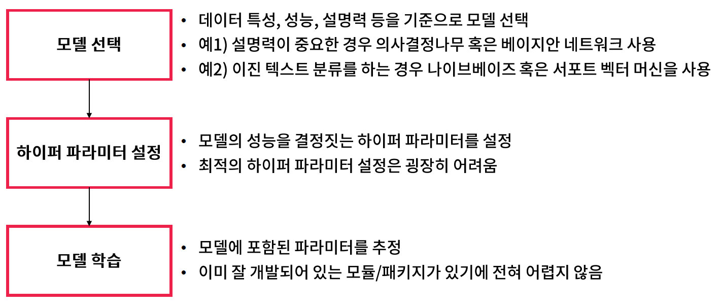
// 모델선택+하이퍼 파라미터 설정은 하나의 단계로 봐도 무방하다.

* 모델평가

 - 분류 모델의 대표적인 지표

  . 정확도 (accuracy) : 전체 샘플 가운데 제대로 예측한 샘플의 비율

  . 정밀도 (precision) : 긍정 클래스라고 에측한 샘플 가운데 실제 긍정 클래스 샘플의 비율

  . 재현율 (recall) : 실제 긍정 클래스 샘플 가운데 제대로 예측된 샘플의 비율

  . F1 점수 (F1-score) : 정밀도와 재현율의 조화 평균

 - 에측 모델의 대표적인 지표

  . 평균 제곱 오차 (mean sqaured erro)

  . 평균 절대 오차 (mean absolute error)

  . 평균 절대 퍼센트 오차 (mean absolute percentage error)

// 평균 절대 퍼센트 오차는 실제로는 잘 안 쓰인다. 분모가 0이 되는 경우가 있다.

 - 잘못된 평가를 피하기 위해, 둘 이상의 평가 지표를 쓰는 것이 바람직하다.

* 결과보고서 작성

 - 지금까지의 분석 결과를 바탕으로 보고서를 작성하는 단계

 - 결과보고서의 통일된 구성은 없지만, 일반적으로 다음과 같이 구성된다.

  1) 분석 목적

  2) 데이터 탐색 및 전처리

  3) 분석 방법

  4) 분석 결과 및 활용 방안

// 어떻게 활용할 것인가가 중요하다.

* 부적절한 문제 정의

// 문제정의가 잘 못 되면 뒤에 결과까지 부적절한 영향을 주게 된다.

 - 부적절한 문제 정의의 가장 흔한 유형으로는 (1) 구체적이지 않은 문제 정의, (2) 부적절한 특징 정의, (3) 수집 불가한 데이터 정의가 있다.

// 3 번의 경우 입문자에게 많이 발생 한다.

 - 타이어 A사 사례

  . 문제 정의 : "타이어 생산 공정에서 발생하는 데이터를 바탕으로 공정을 최적화하고 싶다"

  . 제공 데이터 : 생산 공정에서 발생한 거의 모든 데이터

// 최적화라는 단어가 굉장히 모호한 단어이다. 추상적이다.

// 구체적으로 말할 수 있어야 한다.

// 타이어 생산 공정이라는 자체도 모호하다. 1단계만 이뤄진 것이 아니기 때문이다.

// column 에 대해서 데이터 설명서를 요청했지만 기업도 모른다고 답변을 했었다.

// 컬럼에 대한 정확한 정보를 알고 있어야 한다.

 - 카드 A사 사례

  . 문제 정의 : "일별 콜수요를 예측하고 싶다"

  . 특징 : (1) 상담원 수, (2) 상담원의 역량

// 일별로 상담원수가 바뀔 가능성이 거의 없다.

// 다시 말해서 1, 2번의 변수가 영향을 미치지 않는다.

// 역량을 측정하는 것 자체도 모호하다.

* 부적절한 데이터 수집

 - 부적절한 데이터 수집의 가장 흔한 유형으로 (1) 측정 오류 등으로 수집한 데이터가 실제 상황을 반영하지 못하는 경우, (2) 해결하고자 하는 문제와 무관한 데이터를 수집한 경우, (3) 특정 이벤트가 데이터에 누락된 경우가 있다.

// 데이터 수집이 잘 못 되면 어떤 방법을 쓰더라도 좋은 성능을 얻을 수가 없다.

 - 자동차 시트 A사 사례

  . 배경 : 자동차 시트 폼을 보관하는 과정에서 창고의 온도 및 습도 등에 따라, 폼이 수축하기도 이완하기도 한다.

  . 문제 정의 : 창고의 환경에 따른 폼의 수축 및 이완정도를 예측하고, 그 정도가 심할 것이라 판단되면 환경을 제어

  . 수집데이터 : 창고의 환경 조건과 폼의 수축 / 이완 정도 데이터 (수집 시기 : 2015년 6월 ~8월)

// 문제정의까지는 괜찮았던 정의 단계를 내렸지만...

// 수집데이터의 시기가 6~8월 정도로 이완 정도는 예측 할 수는 있지만, 수축 등의 데이터를 볼 수 없다.

// 통계적인 방향에서 보면 일어나지 않은.. 측정되지 않은 문제는 분석 할 수 없다는 것이다.

// 시기를 겨울철에도 모아서 다시 분석에 활용하였다.

* 부적절한 데이터 탐색

 - 피드백 루프를 발생시키는 핵심 원인이 부적절한 데이터 탐색 혹은 데이터 탐색 생략임

// 탐색을 대충하고, 대충 검정해보고 다시 이전으로 돌아가는 현상이 발생한다.

 - 데이터 탐색을 제대로 하지 않으면, 적절한 모델 선택 및 전처릴 할 수 없어, 모델 평가 단계에서 좋은 성능을 내는 것이 거의 불가능하다.

 - 자동차 A사 사례

  . 문제 정의 : 서비스 센터로 등록되는 클레임 가운데 안전 관련 클레임을 자동 검출하는 시스템 개발

  . 무적절한 탬색 내용 : 클레임에서 오탈자 및 비표준어가 굉장히 많았지만 빈발 단어의 분포 등 만 확인한다.

  . 결과 : 스펠링 교정 등의 전처리를 생략해서, 검출 성능이 매우 낮은 모델이 학습되어 다시 탐색 단계로 되돌아간다.

// 코드를 실행시키고 결과가 나온 시기가 1주일이 걸렸다. 그렇기 때문에 탐색을 꼼꼼히 해야만 된다.

* 부적절한 데이터 전처리

 - 데이터 전처리는 크게 모델 개발을 위해 필수적인 전처리와 모델 성능 향상을 위한 전처리로 구분된다.

 - 모통 모델 성능 향상을 위한 전처리를 생략해서 이전 단계로 되돌아가는 경우가 가장 흔하다.

// 필수적인 전처리를 반드시 해야 한다. Skip 할 수가 없다.

* 부적절한 모델링 및 모델 평가

 - 모델링에서는 주로 부적절한 모델 및 파라미터 선택으로 잘못되는 경우가 대부분이며, 모델링 자체가 잘못되는 경우는 매우 드물다.

 - 모델 평강가는 적절하지 않은 지표를 사용해서 잘못되는 경우가 대부분이며, 대표적인 사례로 단일 지표만 써서 부적절한 모델을 우수한 모델이라고 판단하는 경우가 있다.

// 실제 긍적의 재현율은 0 % 가 되어 버린다.

// 여러지표를 사용하는 것이 중요한 것이다.

// 클래스 분류형 문제가 있는 경우는 하나의 클래스로 치우쳐 발생되는 현상일 수 있다.

[03. Part 3) Ch 14. 이건 꼭 알아야 해 - 지도 학습 모델의 핵심 개념 - 03. 주요 모델의 구조 및 특성-1]

* 선형 회귀 모델과 정규화 회귀 모델

 - 모델 구조

// 샘플 또는 레코드라고 부른다.

- 비용 함수 : 오차제곱합

// 선형 -> 오차 제곱합

// 정규화 -> 계수에 대한 패널티를 추가 시킨다.

* 선형 회귀 모델과 정규화 회귀 모델

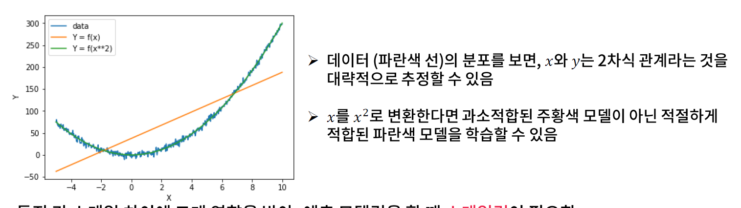
 - 특징과 라벨 간 비선형 관계가 무시될 수 있으므로, 특징 변환이 필요

- 특징 간 스케일 사이에 크게 영향을 받아, 예측 모델링을 할 때 스케일링이 필요하다.

 - 남다 와 max_iter에 따라 과적합 정도가 직접 결정된다.

// max_iter 는 언제까지 학습 시킬 것인가에 대해서 이야기 하는 것이다.

// 신경망 등에서 대해서 고의적으로 작게 잡아서 학습 시킨다. 과적화를 피하기 위해서 그렇게 하는 경우도 있다는 것이다.

* 실습 

// sklearn.linear_model.LinearRegression Documentation

scikit-learn.org/stable/modules/generated/sklearn.linear_model.LinearRegression.html

class sklearn.linear_model.LinearRegression(*, fit_intercept=True, normalize=False, copy_X=True, n_jobs=None)

Ordinary least squares Linear Regression.

LinearRegression fits a linear model with coefficients w = (w1, …, wp) to minimize the residual sum of squares between the observed targets in the dataset, and the targets predicted by the linear approximation.

Parameters

fit_interceptbool, default=True

Whether to calculate the intercept for this model. If set to False, no intercept will be used in calculations (i.e. data is expected to be centered).

normalizebool, default=False

This parameter is ignored when fit_intercept is set to False. If True, the regressors X will be normalized before regression by subtracting the mean and dividing by the l2-norm. If you wish to standardize, please use sklearn.preprocessing.StandardScaler before calling fit on an estimator with normalize=False.

copy_Xbool, default=True

If True, X will be copied; else, it may be overwritten.

n_jobsint, default=None

The number of jobs to use for the computation. This will only provide speedup for n_targets > 1 and sufficient large problems. None means 1 unless in a joblib.parallel_backend context. -1 means using all processors. See Glossary for more details.

Attributes

coef_array of shape (n_features, ) or (n_targets, n_features)

Estimated coefficients for the linear regression problem. If multiple targets are passed during the fit (y 2D), this is a 2D array of shape (n_targets, n_features), while if only one target is passed, this is a 1D array of length n_features.

rank_int

Rank of matrix X. Only available when X is dense.

singular_array of shape (min(X, y),)

Singular values of X. Only available when X is dense.

intercept_float or array of shape (n_targets,)

Independent term in the linear model. Set to 0.0 if fit_intercept = False.

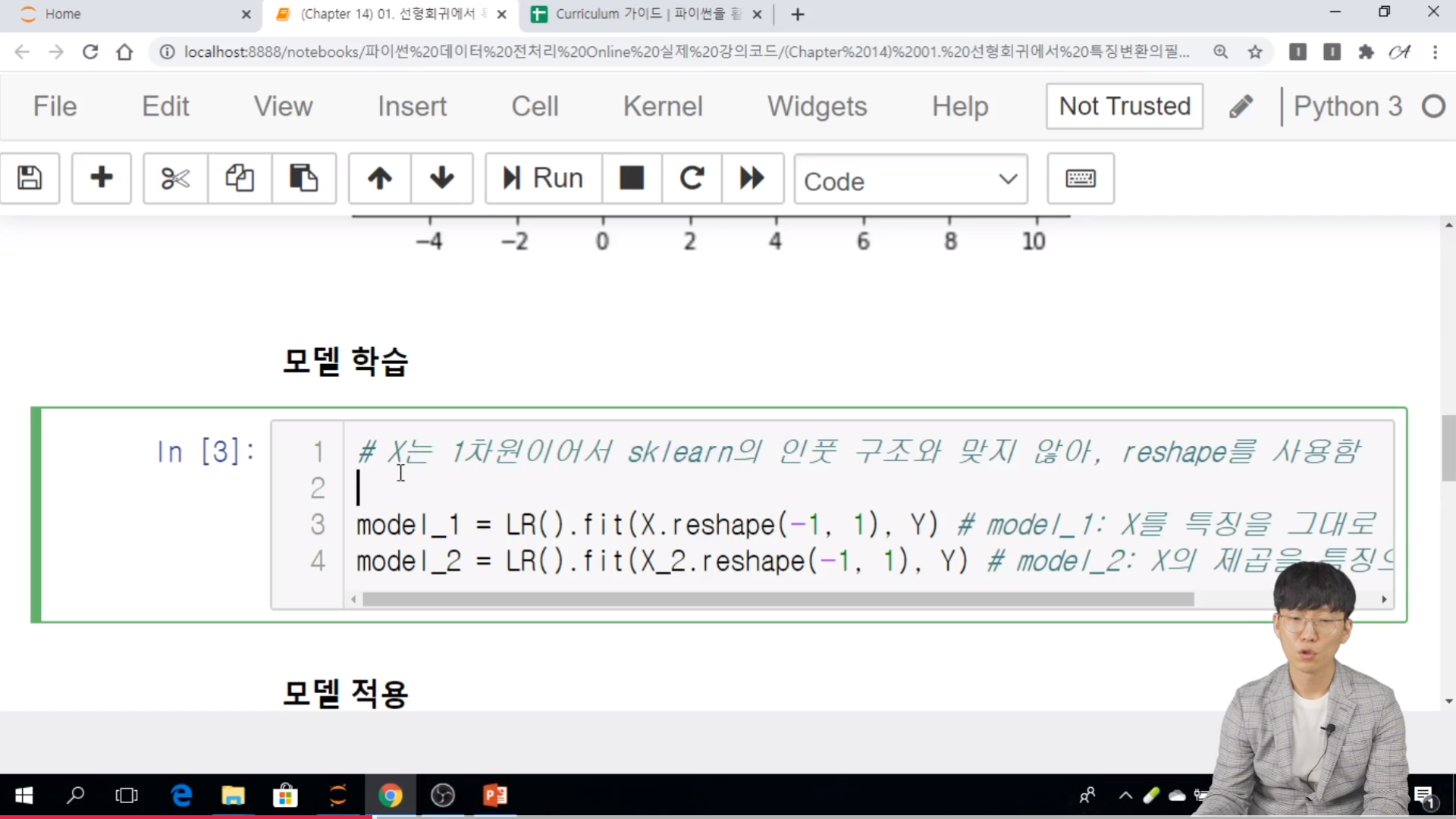
// X는 1차원이어서 sklean 의 인풋 구조와 맞지 않아, reshape를 사용한다.

// 1차원일 경우에는 X=[recod1, record2, ...]

// 학습데이터와 평가 데이터를 나눠야지 정확한 결과가 도출 될 수가 있다.

// 모델링 할 때는 스켈링이 반드시 필요하다. 

* 로지스틱 회귀 모델

// 회귀 모델이지만 분류에 쓰이는 모델이라고 보면 된다.

 - 모델 구조

 - 비용 함수 : 크로스 엔트로피

* 로지스틱 회귀 모델

// 결과적으로는 선형식이라고 보면 된다.

// 선형적인 것들은 아래와 같은 특징을 가진다.

 - 특징의 구간별로 라벨의 분포가 달라지는 경우, 적절한 구간을 나타낼 수 있도록 특징 변환이 필요하다.

* 실습

// 원본을 다시 쓴다고 하면 copy 를 사용한다고 보면 된다.

// sklearn.linear_model.LogisticRegression Documentation

scikit-learn.org/stable/modules/generated/sklearn.linear_model.LogisticRegression.html

class sklearn.linear_model.LogisticRegression(penalty='l2', *, dual=False, tol=0.0001, C=1.0, fit_intercept=True, intercept_scaling=1, class_weight=None, random_state=None, solver='lbfgs', max_iter=100, multi_class='auto', verbose=0, warm_start=False, n_jobs=None, l1_ratio=None)[source]

Logistic Regression (aka logit, MaxEnt) classifier.

In the multiclass case, the training algorithm uses the one-vs-rest (OvR) scheme if the ‘multi_class’ option is set to ‘ovr’, and uses the cross-entropy loss if the ‘multi_class’ option is set to ‘multinomial’. (Currently the ‘multinomial’ option is supported only by the ‘lbfgs’, ‘sag’, ‘saga’ and ‘newton-cg’ solvers.)

This class implements regularized logistic regression using the ‘liblinear’ library, ‘newton-cg’, ‘sag’, ‘saga’ and ‘lbfgs’ solvers. Note that regularization is applied by default. It can handle both dense and sparse input. Use C-ordered arrays or CSR matrices containing 64-bit floats for optimal performance; any other input format will be converted (and copied).

The ‘newton-cg’, ‘sag’, and ‘lbfgs’ solvers support only L2 regularization with primal formulation, or no regularization. The ‘liblinear’ solver supports both L1 and L2 regularization, with a dual formulation only for the L2 penalty. The Elastic-Net regularization is only supported by the ‘saga’ solver.

Read more in the User Guide.

Parameters

penalty{‘l1’, ‘l2’, ‘elasticnet’, ‘none’}, default=’l2’

Used to specify the norm used in the penalization. The ‘newton-cg’, ‘sag’ and ‘lbfgs’ solvers support only l2 penalties. ‘elasticnet’ is only supported by the ‘saga’ solver. If ‘none’ (not supported by the liblinear solver), no regularization is applied.

New in version 0.19: l1 penalty with SAGA solver (allowing ‘multinomial’ + L1)

dualbool, default=False

Dual or primal formulation. Dual formulation is only implemented for l2 penalty with liblinear solver. Prefer dual=False when n_samples > n_features.

tolfloat, default=1e-4

Tolerance for stopping criteria.

Cfloat, default=1.0

Inverse of regularization strength; must be a positive float. Like in support vector machines, smaller values specify stronger regularization.

fit_interceptbool, default=True

Specifies if a constant (a.k.a. bias or intercept) should be added to the decision function.

intercept_scalingfloat, default=1

Useful only when the solver ‘liblinear’ is used and self.fit_intercept is set to True. In this case, x becomes [x, self.intercept_scaling], i.e. a “synthetic” feature with constant value equal to intercept_scaling is appended to the instance vector. The intercept becomes intercept_scaling * synthetic_feature_weight.

Note! the synthetic feature weight is subject to l1/l2 regularization as all other features. To lessen the effect of regularization on synthetic feature weight (and therefore on the intercept) intercept_scaling has to be increased.

class_weightdict or ‘balanced’, default=None

Weights associated with classes in the form {class_label: weight}. If not given, all classes are supposed to have weight one.

The “balanced” mode uses the values of y to automatically adjust weights inversely proportional to class frequencies in the input data as n_samples / (n_classes * np.bincount(y)).

Note that these weights will be multiplied with sample_weight (passed through the fit method) if sample_weight is specified.

New in version 0.17: class_weight=’balanced’

random_stateint, RandomState instance, default=None

Used when solver == ‘sag’, ‘saga’ or ‘liblinear’ to shuffle the data. See Glossary for details.

solver{‘newton-cg’, ‘lbfgs’, ‘liblinear’, ‘sag’, ‘saga’}, default=’lbfgs’

Algorithm to use in the optimization problem.

• For small datasets, ‘liblinear’ is a good choice, whereas ‘sag’ and ‘saga’ are faster for large ones.

• For multiclass problems, only ‘newton-cg’, ‘sag’, ‘saga’ and ‘lbfgs’ handle multinomial loss; ‘liblinear’ is limited to one-versus-rest schemes.

• ‘newton-cg’, ‘lbfgs’, ‘sag’ and ‘saga’ handle L2 or no penalty

• ‘liblinear’ and ‘saga’ also handle L1 penalty

• ‘saga’ also supports ‘elasticnet’ penalty

• ‘liblinear’ does not support setting penalty='none'

Note that ‘sag’ and ‘saga’ fast convergence is only guaranteed on features with approximately the same scale. You can preprocess the data with a scaler from sklearn.preprocessing.

New in version 0.17: Stochastic Average Gradient descent solver.

New in version 0.19: SAGA solver.

Changed in version 0.22: The default solver changed from ‘liblinear’ to ‘lbfgs’ in 0.22.

max_iterint, default=100

Maximum number of iterations taken for the solvers to converge.

multi_class{‘auto’, ‘ovr’, ‘multinomial’}, default=’auto’

If the option chosen is ‘ovr’, then a binary problem is fit for each label. For ‘multinomial’ the loss minimised is the multinomial loss fit across the entire probability distribution, even when the data is binary. ‘multinomial’ is unavailable when solver=’liblinear’. ‘auto’ selects ‘ovr’ if the data is binary, or if solver=’liblinear’, and otherwise selects ‘multinomial’.

New in version 0.18: Stochastic Average Gradient descent solver for ‘multinomial’ case.

Changed in version 0.22: Default changed from ‘ovr’ to ‘auto’ in 0.22.

verboseint, default=0

For the liblinear and lbfgs solvers set verbose to any positive number for verbosity.

warm_startbool, default=False

When set to True, reuse the solution of the previous call to fit as initialization, otherwise, just erase the previous solution. Useless for liblinear solver. See the Glossary.

New in version 0.17: warm_start to support lbfgs, newton-cg, sag, saga solvers.

n_jobsint, default=None

Number of CPU cores used when parallelizing over classes if multi_class=’ovr’”. This parameter is ignored when the solver is set to ‘liblinear’ regardless of whether ‘multi_class’ is specified or not. None means 1 unless in a joblib.parallel_backend context. -1 means using all processors. See Glossary for more details.

l1_ratiofloat, default=None

The Elastic-Net mixing parameter, with 0 <= l1_ratio <= 1. Only used if penalty='elasticnet'. Setting l1_ratio=0 is equivalent to using penalty='l2', while setting l1_ratio=1 is equivalent to using penalty='l1'. For 0 < l1_ratio <1, the penalty is a combination of L1 and L2.

Attributes

classes_ndarray of shape (n_classes, )

A list of class labels known to the classifier.

coef_ndarray of shape (1, n_features) or (n_classes, n_features)

Coefficient of the features in the decision function.

coef_ is of shape (1, n_features) when the given problem is binary. In particular, when multi_class='multinomial', coef_ corresponds to outcome 1 (True) and -coef_ corresponds to outcome 0 (False).

intercept_ndarray of shape (1,) or (n_classes,)

Intercept (a.k.a. bias) added to the decision function.

If fit_intercept is set to False, the intercept is set to zero. intercept_ is of shape (1,) when the given problem is binary. In particular, when multi_class='multinomial', intercept_ corresponds to outcome 1 (True) and -intercept_ corresponds to outcome 0 (False).

n_iter_ndarray of shape (n_classes,) or (1, )

Actual number of iterations for all classes. If binary or multinomial, it returns only 1 element. For liblinear solver, only the maximum number of iteration across all classes is given.

Changed in version 0.20: In SciPy <= 1.0.0 the number of lbfgs iterations may exceed max_iter. n_iter_ will now report at most max_iter.

[03. Part 3) Ch 14. 이건 꼭 알아야 해 - 지도 학습 모델의 핵심 개념 - 03. 주요 모델의 구조 및 특성-2]

* k- 최근접 이웃 (k-Nearest Neighbors; kNN)

 - 모델 구조

* k - 최근접 이웃 (k-Nearest Neighbors ; kNN)

 - 주요 파라미터와 설정 방법

  . 이웃 수 (k) : 홀수로 설정하며, 특징 수 대비 샘플 수가 적은 경우에는 k를 작게 설정하는 것이 바람직하다.

// 홀수로 설정하는 이유는 동점을 방지하기 위해서이다.

// 샘플수가 작다는 것은 데이터가 밀도가 작다는 것이다.

  . 거리 및 유사도 척도

   .. 모든 변수가 서열형 혹은 정수인 경우 : 맨하탄 거리

   .. 방향성이 중요한 경우 (예 : 상품 추천 시스템) : 코사인 유사도

   .. 모든 변수가 이진형이면서 희소하지 않은 경우 : 매칭 유사도

   .. 모든 변수가 이진형이면서 희소한 경우 : 자카드 유사도

   .. 그 외 : 유클리디안 거리

// 희소하다는 것은 데이터 들이 0으로 이뤄져있다고 보면 된다. 텍스트 데이터가 그렇게 이뤄져 있다고 보면 된다.

 - 특징 추출이 어려우나 유사도 및 거리 계산만 가능한 경우 (예: 시퀀스 데이터) 에 주로 활용

 - 모든 특징이 연속형이고 샘플 수가 많지 않은 경우에 좋은 성능을 보인다고 알려져 있음

 - 특징 간 스케일 차이에 크게 영향을 받아, 스케일링이 반드시 필요함 (코사인 유사도를 사용하는 경우 제외)

 - 거리 및 유사도 계산에 문제가 없다면, 별다른 특징 변환이 필요하지 않다.

* 의사 결정 나무 (Decision tree)

 - 모델 구조

// 설명력이 굉장히 높다는 것이 이 의사결정나무의 핵심이라고 볼 수 있다.

 - 예측 과정을 잘 설명할 수 있다는 장점 덕분에 많은 프로젝트에서 활용

  . A 보험사 : 고객의 이탈 여부를 예측하고, 그 원인을 파악해달라

  . B 밸브사 : 밸브의 불량이 발생하는 공정 상의 원인을 파악해달라

  . C 홈쇼핑사 : 방송 조건에 따라 예측한 상품 매출액 기준으로 방송 편성표를 추천해주고, 그 근거를 설명해 달라

 - 선형 분류기라는 한계로 예측력이 좋은 편에 속하지는 못하나, 최근 각광 받고 있는 앙상블 모델 (예 : XGBoost, lightGBM) 의 기본 모형으로 사용된다.

// 예측력은 좋을지 몰라도 설명력이 떨어진다는 문제가 있다.

 - 주요 파라미터

  . max_depth : 최대 깊이로 그 크기가 클수록 모델이 복잡해진다.

  . min_samples_leaf : 잎 노드에 있어야 하는 최소 샘플 수로, 그 크기가 작을 수록 모델이 복잡해진다.

* 나이브 베이즈 (Navie Bayes)

 - 모델 구조

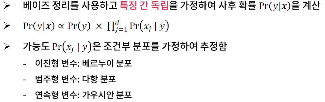
  . 베이즈 정리르 사용하고 특징 간 독립을 가정하여 사후 확률을 계산

  . 가능도는 조건부 분포를 가정하여 추정한다.

   .. 이진형 변수 : 베르누이 분포

   .. 범주형 변수 : 다항 분포

   .. 연속형 변수 : 가우시안 분포

 - 모델 특성

  . 특징 간 독립 가정이 실제로는 굉장히 비현실적이므로, 일반적으로 높은 성능을 기대하긴 어렵다.

// 특징 간 독립 가정이 통계학적으로는 많이 쓰이지만.. 높은 성능을 기대하긴 어렵다.

  . 설정한 분푸에 따라 성능 차이가 크므로, 특징의 타입이 서로 같은 경웨 사용하기 바람직하다.

  . 특징이 매우 많고 그 타입이 같은 문제 (예: 이진형 텍스트 분류)에 주로 사용된다.

  . 특징 간 독립 가정이 실제로는 굉장히 비현실적이므로, 일반적으로 높은 성능을 기대하긴 어렵다.

  . 설정한 분포에 따라 성능 차이가 크므로, 특징의 타입이 서로 같은 경우에 사용하기 바람직하다.

  . 특징이 매우 많고 그 타입이 같은 문제 (예: 이진형 텍스트 분류) 에 주로 사용된다.

* 서포트 벡터 머신 (Support Vector Machine; SVM)

 - 모델 구조

 - 최적화 모델

 - 오차를 최소화하면서 동시에 마진을 최대화하는 분류 모델로, 커널 트릭을 활용하여 저차원 공간을 고차원 공간으로 매핑한다.

 - 마진의 개념을 회귀에 활용한 모델을 서포트 벡터 회귀 (Support Vector Regression)이라 한다.

 - 주요 파라미터

  . kernel : 통상적으로 이진 변수가 많으면 linear 커널이, 연속 변수가 많으면 rbf 커널이 잘 맞는 다고 알려져 있다.

// 특징간 차이는 rbf, 특징간 곱 linear

  . C : 오차 패널티에 대한 계수로, 이 값이 작을 수록 마진 최대화에 클수록 학습 오차 최소화에 신경을 쓰며, 보통 10n 범위에서 튜닝한다.

  . r : rbf 커널의 파라미터로, 크면 클수록 데이터의 모양을 잡 잡아내지만 오차가 커질 위험이 있으며, C 가 증가하면 r도 증가하게 튜닝하는 것이 일반적이다.

 - 파라미터 튜닝이 까다로운 모델이지만, 튜닝만 잘하면 좋은 성능을 보장하는 모델이다.

// 학술에 관심이 있으면 VC 정리...를 확인해보면 좋다.

* 신경망 (Neural Network)

 - 모델 구조

 - 초기 가중치에 크게 영향을 받는 모델로, 세밀하게 random_state 와 max_iter 값을 조정해야 하다.

// 우연에 많이 기반한다는 의미이다. 데이터가 작으면 작을 수록 그런 경향이 크다.

 - 은닉 노드가 하나 추가되면 그에 따라 하나 이상의 가중치가 추가되어, 복잡도가 크게 증가할 수 있다.

 - 모든 변수 타입이 연속형인 경우에 성능이 잘 나오는 것으로 알려져 있으며, 은닉 층 구조에 따른 복잡도 조절이 파라미터 튜닝에서 고려해야 할 가장 중요한 요소임

 - 최근 딥러닝의 발전으로 크게 주목받는 모델이지만, 특정 주제 (예 : 시계열 예측, 이미지 분류, 객체 탐지 등) 를 제외하고는 깊은 층의 신경망은 과적합으로 인한 성능 이슈가 자주 발생한다.

* 트리 기반의 앙상블 모델

 - 최근 의사 결정나무를 기본 모형으로 하는 앙상블 모형이 캐글 등에서 자주 사용되며, 좋은 성능을 보인다.

 - 랜덤 포레스트 : 배깅(bagging) 방식으로 여러 트리를 학습하여 결합한 모델

 - XGboost & LightGBM : 부스팅 방식으로 여러 트리를 순차적으로 학습하여 결합한 모델

 - 랜덤 포레스트를 사용할 때는 트리의 개수와 나무의 최대 깊이를 조정해야 하며, XGboost 와 LightGBM 을 사용할 때는 트리의 개수, 나무의 최대 깊이, 학습률을 조정해야 한다.

  . 트리의 개수 : 통상적으로 트리의 개수가 많으면 많을 수록 좋은 성능을 내지만, 어느 수준 이상에서는 거의 큰 차일ㄹ 보이지 않는다.

  . 나무의 최대 깊이 : 4이하로 설정해주는 것이 과적합을 피할 수 있어, 바람직하다.

  . 학습률 : 이 값은 작으면 작을 수록 과소적합 위험이 있으며, 크면 클수록 과적합 위험이 있다. 통상적으로 0.1로 설정한다.

[파이썬을 활용한 데이터 전처리 Level UP-Comment]
- 모델 개발 프로세스에 대해서 배웠고, 지도학습에서는 선형회귀, 의사결정나무, 신경망 등에 대해서도 배워 볼 수 있었다.

https://bit.ly/3m7bW22

[파이썬을 활용한 데이터 전처리 Level UP- 20 회차 미션 시작]

* 복습

 - 홈페이지 분석을 위한 데이터 불러오기, 검정 방법, p-value 값에 대한 해석에 대해서 알아보았다.

[02. Part 2) Ch 13. 직접 해봐야 내것이 된다. - 02. 고객 세분화를 통한 마케팅 전략 수립 (실습)]

// 데이터 분할

// 각각의 Quantity 에서 음수를 구분해야 한다.

// 환불 데이터와, 주문 데이터를 각각 구분한다.

// 고객별 특징 추출

// 클러스터링을 위해서 데이터 초기화를 해야 한다.

// unique( ) 을 통해서 dataframe 을 만들어 준다.

// 주문 횟수 계산 및 부착을 한다.

// value_counts( ) 를 통해서.. 한 주문에서 여러개의 상품을 구매하기 때문에 CustomerID, InvoiceNo 로 분류 해준다.

// 시리즈로 만들어진 데이터를 to_dict( ) 로 바꾸어 준다. key 사전 id. value 주문횟수

// 주문 횟수가 0인 경우에는 replace 가 되지 않아 Customer ID 가 부착될 수 있다.

// 이러한 경우를 대비하기 위해서 0으로 변경한다.

// 반품 횟수에 대서 계산 및 부착

// 위와 동일 한 방법으로 주문횟수와 반품 횟수로 변경해준다.

// 주문량 계산 및 부착을 해준다.

// 주문 금액 합계 계산 및 부착

// Quantity 와 UnitPrice 로 주문금액을 만들어준다.

// 이 상태에서 최근 주문과 현재 시점까지의 거리를 부착해준다.

// to_datetime( ) 찾아보기

// pandas.to_datetime Documentation

pandas.pydata.org/pandas-docs/stable/reference/api/pandas.to_datetime.html

pandas.to_datetime(arg: DatetimeScalar, errors: str = '...', dayfirst: bool = '...', yearfirst: bool = '...', utc: Optional[bool] = '...', format: Optional[str] = '...', exact: bool = '...', unit: Optional[str] = '...', infer_datetime_format: bool = '...', origin='...', cache: bool = '...') → Union[DatetimeScalar, ‘NaTType’]
pandas.to_datetime(arg: ‘Series’, errors: str = '...', dayfirst: bool = '...', yearfirst: bool = '...', utc: Optional[bool] = '...', format: Optional[str] = '...', exact: bool = '...', unit: Optional[str] = '...', infer_datetime_format: bool = '...', origin='...', cache: bool = '...') → ’Series’
pandas.to_datetime(arg: Union[List, Tuple], errors: str = '...', dayfirst: bool = '...', yearfirst: bool = '...', utc: Optional[bool] = '...', format: Optional[str] = '...', exact: bool = '...', unit: Optional[str] = '...', infer_datetime_format: bool = '...', origin='...', cache: bool = '...') → DatetimeIndex

Convert argument to datetime.

Parameters

argint, float, str, datetime, list, tuple, 1-d array, Series, DataFrame/dict-like

The object to convert to a datetime.

errors{‘ignore’, ‘raise’, ‘coerce’}, default ‘raise’

• If ‘raise’, then invalid parsing will raise an exception.

• If ‘coerce’, then invalid parsing will be set as NaT.

• If ‘ignore’, then invalid parsing will return the input.

dayfirstbool, default False

Specify a date parse order if arg is str or its list-likes. If True, parses dates with the day first, eg 10/11/12 is parsed as 2012-11-10. Warning: dayfirst=True is not strict, but will prefer to parse with day first (this is a known bug, based on dateutil behavior).

yearfirstbool, default False

Specify a date parse order if arg is str or its list-likes.

• If True parses dates with the year first, eg 10/11/12 is parsed as 2010-11-12.

• If both dayfirst and yearfirst are True, yearfirst is preceded (same as dateutil).

Warning: yearfirst=True is not strict, but will prefer to parse with year first (this is a known bug, based on dateutil behavior).

utcbool, default None

Return UTC DatetimeIndex if True (converting any tz-aware datetime.datetime objects as well).

formatstr, default None

The strftime to parse time, eg “%d/%m/%Y”, note that “%f” will parse all the way up to nanoseconds. See strftime documentation for more information on choices: https://docs.python.org/3/library/datetime.html#strftime-and-strptime-behavior.

exactbool, True by default

Behaves as: - If True, require an exact format match. - If False, allow the format to match anywhere in the target string.

unitstr, default ‘ns’

The unit of the arg (D,s,ms,us,ns) denote the unit, which is an integer or float number. This will be based off the origin. Example, with unit=’ms’ and origin=’unix’ (the default), this would calculate the number of milliseconds to the unix epoch start.

infer_datetime_formatbool, default False

If True and no format is given, attempt to infer the format of the datetime strings based on the first non-NaN element, and if it can be inferred, switch to a faster method of parsing them. In some cases this can increase the parsing speed by ~5-10x.

originscalar, default ‘unix’

Define the reference date. The numeric values would be parsed as number of units (defined by unit) since this reference date.

• If ‘unix’ (or POSIX) time; origin is set to 1970-01-01.

• If ‘julian’, unit must be ‘D’, and origin is set to beginning of Julian Calendar. Julian day number 0 is assigned to the day starting at noon on January 1, 4713 BC.

• If Timestamp convertible, origin is set to Timestamp identified by origin.

cachebool, default True

If True, use a cache of unique, converted dates to apply the datetime conversion. May produce significant speed-up when parsing duplicate date strings, especially ones with timezone offsets. The cache is only used when there are at least 50 values. The presence of out-of-bounds values will render the cache unusable and may slow down parsing.

New in version 0.23.0.

Changed in version 0.25.0: - changed default value from False to True.

Returns

datetime

If parsing succeeded. Return type depends on input:

• list-like: DatetimeIndex

• Series: Series of datetime64 dtype

• scalar: Timestamp

In case when it is not possible to return designated types (e.g. when any element of input is before Timestamp.min or after Timestamp.max) return will have datetime.datetime type (or corresponding array/Series).

// recency 로 날짜를 처리한다.

// 하나의 element를 처리 한다는 것이다.

// keep = last 를 통해서, 계산량을 감소 시키는 것이다.

// keep 을 last 로 두는 이유는 맨 마지막 값을 두기 위한 것이다.

// CustomerID, Invoice 데이터를 가지고 오고.. 이건 최근성 이라는 column에 넣어준다.

// 각각의 스케일이 틀리기 때문에 유클리디안 거리등을 사용하기는 어렵다.

// 고객의 주문 특성에 따라서 군집화를 수행하다.

// 군집화 모델을 인스터스화 하고 학습을 시켜준다.

// 각각의 데이터를 보고 확인해 본다.

// 주요 상품에 대해서 확인을 해본다.

// TransactionEncdoer 를 통해서 나타내본다.

// 희소한지를 알아봐야 한다.

// 여기서 모든 것을 사용하는 것은 아니고 빈도가 100회 이상 나온 품목만 사용하면 된다.

// 차원을 줄여서 확인을 해 봐야 한다.

[02. Part 2) Ch 13. 직접 해봐야 내것이 된다. - 03. 이탈 고객의 고객 여정 탐색하기]

* 문제상황

 - 고객 로그 데이터를 바탕으로 이탈한 고객과 이탈하지 않은 고객이 보이는 주요 행동 패턴을 탐색하자!

  (1) 이탈 고객과 비이탈 고객 분리

  (2) 이탈 고객과 비이탈 고객 데이터 내 주요 행동 패턴 추출

  (3) 주요 행동 패턴의 등장 비율 비교

* 실습

// sort_values 를 통해서 고객ID, 날짜로 가져오고

// 행동을 unique 상태로 확인하고

// 다른 행동이 있을 수 있기 때문에 ~ not( churn_ID 에 속하지 않는 ID 를 찾아 본다.)

// isin 함수를 통해서 확인

// 이탈이든 아니든 고객ID 의 행동에 따라서 array 형태로 나타낸다.

// 비말 패턴 탐색에서 사용했던 함수들을 가지고 와서 빈말 패턴을 찾아 본다.

[03. Part 3) Ch 14. 이건 꼭 알아야 해 - 지도 학습 모델의 핵심 개념 - 01. 지도학습 개요]

// 기초적인 내용은 생략되어 있다.~

* 지도 학습

 - 컴퓨터에게 입력과 출력을 주고, 입력과 출력 간 관계를 학습하여 새로운 입력에 대해 적절한 출력을 내도록 하는 기계학습의 한 분야

 - 입력을 특징(feature) 혹은 특징 벡터 (featur vector)라고 하며, 출력을 라벨 (label)이라고 함

// 특징과 라벨간의 관계를 학습하는 거라고 보면 된다.

 - 라벨이 범주형 변수면 분류라고 하며, 연속형 변수면 예측 혹은 회귀라고 한다.

* 과적합

 - 지도학습 모델은 학습 데이터를 분류하고 예측하는 수준으로, 학습에 사용되지 않은 데이터도 정확히 분류하고 예측하리라 기대하며, 이러한 기대가 충족되는 경우 일반화 되었다고 한다.

 - 모델이 너무 족잡해서 학습 데이터에 대해서만 정확히 분류하고 예측하는 모델을 과적합되었다고 하며, 반대로 너무 단순해서 어떠한 데이터에 대해서도 부적합한 모델을 과소적합되었다고 한다.

// 적정적합은 오차가 조금씩 있고, 과적합은 오차가 전혀 없는 상태로 본다.

// 적정적합은 학습 데이터를 사용해서 학습을 했을 것이고.. 과적합은 너무 복잡하게 되어 있어서 데이터에 대해서만 과하게 적합이라고 보면 된다.

- 과적합과 과소적합에 영향을 끼치는 주요 인자로는 모델의 복잡도, 샘플 수, 차원의 크기 등이 있다.

// 샘플수는 이 모델을 지지하는 근거하는.. 수라고 보면 된다.

// 적으면 성급한 일반화가 되어 버릴 수가 있다.

* 데이터 분할

 - 과적합된 모델을 좋게 평가하는 것을 방지하기 위해서, 데이터를 학습 데이터와 평가 데이터로 분할한다.

// 객관적인 결과를 위해서 평가 데이터를 모르게 해야 한다.

 - 학습 데이터와 평가 데이터가 지나치게 유사하거나 특정 패턴을 갖지 않도록 분할 해야 한다.

* 파라미터와 하이퍼 파라미터

 - 하이퍼 파라미터(hyper parameter)는 일종의 사용자 옵션으로, 모델 성능에 직접적으로 영향을 끼치므로 자세한 데이터 탐색 결과를 바탕으로 선택해야 한다.

// 파라미터는 신경을 많이 쓰지 않는다고 보면 된다.

// 머신러닝에서 무조건 좋다는 것은 없다고 보면 된다. 경험으로 이것이 좀 더 나아 보인다고 생각하면 된다.

* 이진 분류 모델 평가 : 혼동 행렬

 - 이진 분류 : 클래스 변수의 상태 공간이 크기가 2인 분류

// 상태 공간은 값의 갯수로 보면 된다.

 - 혼동 행렬 : 분류 모델을 평가하는데 사용하는 표

  . Positive class : 분석의 관심 대상 (보통 1로 설정)

  . Negativ class : 분석 관심 대상 외 (보통 0이나 -1로 설정)

* 이진 분류 모델 평가 : 대표적인 지표

 - 각 지표의 한계 때문에, 가능한 여러 지표를 사용하여 모델을 평가해야 한다.

// 정확도 가 가장 많이 쓰이고, 공정하고

// F1 은 정확도랑 전혀 관계가 없다고 생각해야 한다.

* 다중 분류 모델 평가

 - 다중 분류 : 클래스 변수의 상태 공간이 크기가 3이상인 분류

 - 각 클래스를 긍정으로 간주하여 평가 지표를 계산한 뒤, 이들의 산술 평균이나 가중 평균으로 평가

// 산술 평균 marco average

// 가중 평균 weight average

* 예측 모델 평가

 - 대표적인 예측 모델 평가 지표로 루트 평균 제곱 오차 (root mean squared erro ;  RMSE) 와 평균 절대 오차 (mean absolute error ; MAE) 가 있으며, 두 지표 모두 값이 작을 수록 좋음

 - RMSE 와 MAE를 정확히 평가하려면, 해당 분야의 도메인 지식이나 클래스 변수의 스케일을 고려해야 한다.

  . 예를 들어, 코스피 지수를 예측하는 모델의 MAE 가 1010 이라면 무의미한 수준의 모델이지만, 전세계 인구 수를 예측하는 모델의 MAE 가 1010 이라면 매우 우수한 모델이다.

[파이썬을 활용한 데이터 전처리 Level UP-Comment]
- 고객 데이터 활용 실습을 해보았고, 고객 이탈 여정에 대해서 간략하게 다른 주제로 살펴 볼 수 있었다. 지도 학습에 대한 주요 개념들을 배웠다.

https://bit.ly/3m7bW22

[파이썬을 활용한 데이터 전처리 Level UP- 19 회차 미션 시작]

* 복습

 - 빈발 패턴, 머신러닝에서의 활용, 어떤식을 구성을하면 소비자들이 더 머물고, 다른 전환율이 많이 발생할지에 대해서 알아보았다.

[02. Part 2) Ch 13. 직접 해봐야 내것이 된다. - 01. A-B 테스트 - 홈페이지 화면을 어떻게 구성할 것인가 - (실습 - Step 1 ~ 2)]

// %matplotlib inline 그래프 그리기 위한

// plt.rcParams 를 통해서 각각의 옵션을 정해서 나타낸다.

// 1년치 데이터라서 위치를 찾기 어렵기 때문에

// 월별 일 수 누적을 통한 매월 1일 인덱스 정의 (12월 제외) 했다.

// xtick_range = np.cumsum 을 통해서 확인함.

// 변동 자체는 그렇게 확 띄거나 변동성이 많이 없는 것 같다.

Step 2. 상품 배치와 상품 구매 금액에 따른 관계 분석

// index_col 을 사용해서 불러올때 부터 고객 ID 로 index 를 설정하는 것이다.

// 이런식으로 placement_A, placement_B, placement_C

// 원래는 같은 고객을 불러 오는 것이 더 좋을 수도 있다.

// 정확한 테스트를 위해서는 고객 ID 가 일치하는 것이 더 좋다.

// 현실적으로는 다른 고객들을 불러 온다.

// 구매금액이 0인 고객들을 제외하고 필터링

placement_A_without_zero = placement_Aloc[placement_A['구매금액'] != 0]['구매금액'].values

// ndarray 형태로 불러왔다. 뒤에 있는 scipy.stats 를 잘 사용하기 위해서 이런 형태로 불러 온것이다.

// 각 데이터가 정규 분포를 따름을 확인하는 과정

// scipy.stats 를 통해서 어떤 종류인지를 확인한다.

// 일원분산분석 수행을 한다.

// p-value 가 거의 -에 수렴 => A, B, C의 평균은 유의한 차이가 존재

// 이런 상태이기 때문에 사후 분석을 진행했다.

// from statsmodels.stats.multicomp import pairwise_tukeyhsd

// (A, C) ~ B 의 관계임을 확인한다.

// A, C 가 비슷하고 B 가 다르다는 것을 확인할 수 있다.

// 각 데이터가 정규분포를 따르는 것을 확인하고

// 다시 같은 방법으로 확인한다.

// A B 가 차이가 있고, A C, B C 가 차이가 없다.

// 이번에는 A ~ (B, C) 관계임을 확인 할 수 있다.

// 구매 여부와 상품 배치 간 관계 파악

// 각각의 데이터를 사용하기 위해서 데이터를 변환, index 가 겹칠 일이 없기 때문에 ignore_index = False 로 두었다.

// 0 이면 구매를 하지 않은것 구매 금액을 체크해서 그걸 boolean 을 다시 astype(int) 을 사용해서 0과 1로 변환한다.

// 데이터를 합친 이유는 범주형 을 분석. 즉, 카이제곱 검정을 하기 위해서 이렇게 사용하였다.

// p-value 가 0.06으로 구매여부와 상품배치에는 관계가 있다고 보기 힘들다.

[02. Part 2) Ch 13. 직접 해봐야 내것이 된다. - 01. A-B 테스트 - 홈페이지 화면을 어떻게 구성할 것인가 - (실습 - Step 3 ~ 6)]

// Step 3. 사이트맵 구성에 따른 체류 시간 차이 분석

// 각각의 sitemap 을 불러 오고, 이번에는 index_col 을 불러 오지 않는다.

// boxplot 함수를 사용해서 확인해본다.

// 하나의 box 는 1부터 시작한다. 그래서 plt.xtics 설정

// 정규 분포를 따르는지 우선 확인

// 거의 0 이다.

// 일원분산분석 : p-value 가 0 에 수렴 > A, B, C 가 거의 차이가 없음.

// Step 4. 할인 쿠폰의 효과 분석

// 발행후 구매횟수 에서 발행전 구매 횟수 차이를 구한다.

// .describe( ) 를 통해서 확인해본다.

// std 가 큰것은 이 값이 큰지를 안 큰지를 알 수가 없다. 분석이 필요하다.

// 통계량만 분석만 하면 기계적으로 분석할 위험이 있다. 그래서 그래프를 그려서 확인해본다.

// Step 5. 체류 시간과 구매 금액 간 관계분석

// 체류시간이 길어지면 구매 금액이 커지는지를 확인해본다.

// 이걸 보기 위해서 상황분석이 필요하다.

// 선형에서는 0.32 상관관계를.. 볼 수 있다.

// Step 6. 구매 버튼 배치에 따른 구매율 차이 분석

// fillna 는 결측을 바꾸는 함수이다.

// pandas.DataFrame.fillna Documentation

pandas.pydata.org/pandas-docs/stable/reference/api/pandas.DataFrame.fillna.html

DataFrame.fillna(value=None, method=None, axis=None, inplace=False, limit=None, downcast=None)

Fill NA/NaN values using the specified method.

Parameters

valuescalar, dict, Series, or DataFrame

Value to use to fill holes (e.g. 0), alternately a dict/Series/DataFrame of values specifying which value to use for each index (for a Series) or column (for a DataFrame). Values not in the dict/Series/DataFrame will not be filled. This value cannot be a list.

method{‘backfill’, ‘bfill’, ‘pad’, ‘ffill’, None}, default None

Method to use for filling holes in reindexed Series pad / ffill: propagate last valid observation forward to next valid backfill / bfill: use next valid observation to fill gap.

axis{0 or ‘index’, 1 or ‘columns’}

Axis along which to fill missing values.

inplacebool, default False

If True, fill in-place. Note: this will modify any other views on this object (e.g., a no-copy slice for a column in a DataFrame).

limitint, default None

If method is specified, this is the maximum number of consecutive NaN values to forward/backward fill. In other words, if there is a gap with more than this number of consecutive NaNs, it will only be partially filled. If method is not specified, this is the maximum number of entries along the entire axis where NaNs will be filled. Must be greater than 0 if not None.

downcastdict, default is None

A dict of item->dtype of what to downcast if possible, or the string ‘infer’ which will try to downcast to an appropriate equal type (e.g. float64 to int64 if possible).

Returns

DataFrame or None

Object with missing values filled or None if inplace=True.

[02. Part 2) Ch 13. 직접 해봐야 내것이 된다. - 02 고객 세분화를 통한 마케팅 전략 수립 (문제)]

* 문제상황

 - 주문 내역 데이터를 바탕으로 고객들을 주문 특성과 주문 상품에 따라 그룹화 하고 싶다!

  . 주문 특성 기준 군집화

   -> 환불 데이터와 주문 데이터로 분할

   -> 특징 부착

   -> 코사인 유사도 기반의 계층 군집화 수행

  . 주문 상품 기준 군집화

   -> 판매 상위 100개 상품 출현 여부를 나타내는 데이터로 변환

   -> 자카드 유사도 기반의 계층 군집화 수행

* 주문 특성 기준 군집화 - 데이터 분할

 - 해당 데이터에는 주문 데이터와 환불 데이터가 동시에 포함되어 있다.

 - 환불 데이터는 주문 수량이 음수라는 특징이 있어, 데이터를 분할하는데 활용한다.

// 이런 특징을 이용해서 주문 데이터와 환불 데이터를 분류할 것이다.

* 주문 특성 기준 군집화 - 특징 추출

 1. 군집화 데이터를 유니크한 고객 ID 컬럼만 있는 데이터프레임으로 초기화

 2. 주문 / 반품 횟수 계산 및 부착 : 고객 ID 와 주문 ID 를 기준으로 중복을 제거 하는 방식으로 유니크한 (고객 ID, 주문 ID) 를 추출한 뒤, 추출한 데이터에서 고객 ID 의 수를 카운트하여 군집화 데이터에 부착

 3. 주문량 계산 및 부착 : 고객 ID에 따른 주문량의 합계를 계산하여 군집화 데이터에 부착

 4. 주문 금액 계산 및 부착 : 주문량과 단가를 곱하여 주문 금액을 계산한 뒤, 고객 ID에 따른 주문 금액의 합계를 계산하여 군집화 데이터에 부착

 5. 최근성 계산 및 부착 : 현재 날짜에서 주문 날짜의 차이를 뺀 뒤, 고객별 해당 값의 최소 값을 군집화 데이터에 부착

* 주문 특성 기준 군집화 - 코사인 유사도 기반의 계층 군집화 수행

 - 군집화 데이터에 (군집 개수 = 5, 군집간 거리 = 평균, 거리 척도 = 코사인 유사도)를 갖는 군집화 모델을 학습하여, 군집별 주요 특성을 파악

* 주문 상품 기준 군집화

 - 주문 횟수가 상위 100 등안에 드는 상품들을 기준으로 고객을 상품 구매 여부로 구성된 벡터로 표현

 - 이 데이터에 (군집 개수 = 5, 군집 간 거리 = 평균, 거리 척도 = 자카드 유사도)를 갖는 군집화 모델을 학습하여, 군집별 주요 특성을 파악한다.

// 희소한 데이터에 적절한 유사도 이기때문에 자카드 유사도를 사용했다.

[파이썬을 활용한 데이터 전처리 Level UP-Comment]
- 홈페이지 분석을 위한 데이터 불러오기, 검정 방법, p-value 값에 대한 해석에 대해서 알아보았고, 새로운 실습 주제에 대해서 설명함.

https://bit.ly/3m7bW22

[파이썬을 활용한 데이터 전처리 Level UP- 18 회차 미션 시작]

* 복습

 - 빈발 개념에 대해서 배웠으나 약간의 개념 정리가 필요한 것 같다. 어떤 sequence 를 이뤄서 나타내는 조건들에 대해서 분석을 해보고, 어똔 조건에서 어떠한 결과물을 내놓는 것에 대해서는 좀 더 연구가 필요하지 않나 싶다.

[02. Part 2) Ch 12. 어디서 많이 봤던 패턴이다 싶을 때 - 빈발 패턴 탐색 - 03. 빈발 시계열 패턴 탐색]

* 시계열 데이터란?

 - 시계열 데이터란 각 요소가 (시간, 값) 형태로 구성된 데이터로, 반드시 순서 및 시간을 고려해야 한다.

* 시계열과 시퀀스 데이터의 차이

 - 시계열 데이터와 시퀀스 데이터는 사용하는 인덱스와 값의 종류로 다음과 같이 구분할 수 있다.

 - 다만, 엄밀히 말해서 시계열 데이터도 시퀀스 데이터에 속한다.

// 시퀀스 데이터에 속하기는 하지만 표를 참고하는 것이 더 좋다.

* 시계열 패턴의 정의

 - 시계열의 패턴은 크게 모양, 변화에 의한 패턴과 값에 의한 패턴으로 구분할 수 있다.

 - 계절성 혹은 주기성이 있는 경우를 제외하면, 모양 패턴을 찾는 것은 거의 불가능에 가깝다.

* SAX : 시계열 -> 시퀀스

 - 시계열 데이터는 연속형이라는 특징 때문에 패턴을 찾으려면 이산화가 필요하며, SAX (symbolic aggregate approximatinon) 을 사용하면 시계열 데이터를 효과적으로 이산화할 수 있다.

// 범주화 하기 위한 방법이라고 보면 된다.

 - SAX 는 (1)원도우 분할, (2) 원도우별 대표값 계산, (3) 알파벳 시퀀스로 변환이라는 세 단계로 구성된다.

* 실습

// 날짜가 포함되어 있기 때문에 parse_date = True 로 두고 불러 온다.

// 인덱스가 날짜, 좀더 큰 범위로 시간이라고 보면 된다.

// 다별량 시계열은 하나의 시간에 더 많은 데이터가 붙어 있는 것이다.

// 하나만 있는 것은 단별량 시계열이라고 한다.

// 다별량 시계열의 경우가 더 분석하기 힘들다.

// segmentation 정의하기

// x : time seires sample, w : windows size, a : alphabe size

// 정상적으로 들어가는 window에 대해서만 처리 해주고...

// 행별 평균을 구한다. mean(axis =1 ) => 결과는 반드시 벡터 일 것이다.

// find_break_pints

// 구간의 범위의 기준선들을 의미한다.

// wmv : windows mean vector

// conversion_window 정의

// chr( ) 아시키 코드를 알파벳으로 바꿔주는 것이다.

// python 내장 함수 chr( )

docs.python.org/3/library/functions.html#chr

chr(i)

Return the string representing a character whose Unicode code point is the integer i. For example, chr(97) returns the string 'a', while chr(8364) returns the string '€'. This is the inverse of ord().

The valid range for the argument is from 0 through 1,114,111 (0x10FFFF in base 16). ValueError will be raised if i is outside that range.

@classmethod

Transform a method into a class method.

A class method receives the class as implicit first argument, just like an instance method receives the instance. To declare a class method, use this idiom:

class C:
    @classmethod
    def f(cls, arg1, arg2, ...): ...

The @classmethod form is a function decorator – see Function definitions for details.

A class method can be called either on the class (such as C.f()) or on an instance (such as C().f()). The instance is ignored except for its class. If a class method is called for a derived class, the derived class object is passed as the implied first argument.

Class methods are different than C++ or Java static methods. If you want those, see staticmethod() in this section. For more information on class methods, see The standard type hierarchy.

Changed in version 3.9: Class methods can now wrap other descriptors such as property().

// 패턴 찾기

// 문자열로 변환 (하나의 리스트만 대상으로 하기에, 이렇게 하는 것이 더 수월)

// join 으로 각 alphabet 을 붙여줌.

// find_maximum_frequent_sequence_item 함수

// 각각의 신뢰도와 지지도를 확인해 볼 수 있다.

[02. Part 2) Ch 12. 어디서 많이 봤던 패턴이다 싶을 때 - 빈발 패턴 탐색 - 04. 머신러닝에서의 빈발 패턴 탐색]

* 추천 시스템

 - "상품 A 를 구매하면 상품 B 도 구매할 것이다" 라는 유의한 연관 규칙이 있다면, 상품 A 를 구매하고 상품 B 를 구매하지 않은 고객에게 상품 B 를 추천해주는 방법에 활용

// 가장 대표적인 것

 - (예시) 아마존의 도서 추천

* 시계열 및 시퀀스 데이터에서의 특징 추출

 - 시계열 및 시퀀스 분류 과제에서 특징을 추출하는데도 활용

// 원도우 크기를 정렬해줘야 한다.

// 지도 학습 또는 비지도 학습에 활용할 수 있다는 점이 있다.

[02. Part 2) Ch 13. 직접 해봐야 내것이 된다. - 01. A-B 테스트 - 홈페이지 화면을 어떻게 구성할 것인가 - (문제)]

* A/B 테스트란?

 - 임의로 나눈 둘 이상의 집단에 서로 다른 컨텐츠를 제시한 뒤, 통계적 가설 검정을 이용하여 어느 컨텐츠에 대한 반응이 더 효과적인지를 파악하는 방법

ko.wikipedia.org/wiki/A/B_%ED%85%8C%EC%8A%A4%ED%8A%B8

A/B 테스트

웹 사이트에서의 A/B 테스트 예제. 한 웹 사이트에서 한 개의 버튼 요소의 디자인만 다른 두 가지 버전을 무작위로 방문자에게 제공해, 두 디자인의 상대적인 효용성을 측정할 수 있다.

마케팅과 웹 분석에서, A/B 테스트(버킷 테스트 또는 분할-실행 테스트)는 두 개의 변형 A와 B를 사용하는 종합 대조 실험(controlled experiment)이다.[1] 통계 영역에서 사용되는 것과 같은 통계적 가설 검정 또는 "2-표본 가설 검정"의 한 형태다. 웹 디자인 (특히 사용자 경험 디자인)과 같은 온라인 영역에서, A/B 테스트의 목표는 관심 분야에 대한 결과를 늘리거나 극대화하는 웹 페이지에 대한 변경 사항이 무엇인지를 규명하는 것이다(예를 들어, 배너 광고의 클릭률(click-through rate)). 공식적으로 현재 웹 페이지에 null 가설과 연관이 있다. A/B 테스트는 변수 A에 비해 대상이 변수 B에 대해 보이는 응답을 테스트하고, 두 변수 중 어떤 것이 더 효과적인지를 판단함으로써 단일 변수에 대한 두 가지 버전을 비교하는 방법이다.[2]

이름에서 알 수 있듯이, 두 버전(A와 B)이 비교되는데 사용자의 행동에 영향을 미칠 수 있는 하나의 변형을 제외하면 동일하다. 버전 A는 현재 사용되는 버전(control)이라고 하는 반면, 버전 B의 일부 사항은 수정된다(treatment). 예를 들어, 전자상거래 웹사이트에서 구매 깔때기은 일반적으로 A/B 테스트하기 좋은 대상으로, 하락률에 있어 수익 한계선에 대한 개선이 판매에 있어 상당한 이익을 나타낼 수 있기 때문이다. 항상 그런 것은 아니지만, 때때로 텍스트, 레이아웃, 이미지 그리고 색상과 같은 요소들을 테스트함으로써 현저한 향상을 볼 수 있다.[3]

다변량 테스트 또는 다항 테스트가 A/B 테스트와 유사하지만, 동시에 두 개 이상의 버전을 테스트하거나 좀 더 많은 컨트롤들을 테스트할 수 있다. 두 개 이상의 버전 또는 동시에 더 많이 사용을 제어한다. 단순한 A/B 테스트는 설문 데이터, 오프라인 데이터 그리고 다른 좀 더 복잡한 현상과 같이, 실측, 유사 실험 또는 기타 비 실험 상황에서는 유효하지 않다.

A/B 테스트는 그 접근 방식이 다양한 연구 관례에서 일반적으로 사용되는, 피험자간 설계와 유사하긴 하지만, 특정 틈새 영역에서 철학과 사업 전략의 변화로 마케팅되었다.[4][5][6] 웹 개발 철학으로서의 A/B 테스트는 해당 영역을 증거 기반의 실천으로의 폭넓은 움직임으로 이끈다. 대부분의 마케팅 자동화 도구가 현재 일반적으로 A/B 테스트를 지속적으로 실행할 수 있는 기능과 함께 제공되고 있기 때문에, A/B 테스트가 거의 모든 영역에서 지속적으로 수행될 수 있는 것으로 간주되는 것이 A/B 테스트의 이점이다. 이로써 현재의 리소스를 사용해 웹 사이트와 다른 도구를 업데이트해 트렌드 변화를 유지할 수 있다.

// 버튼이 어떻게 배치되었을 때 클릭을 많이 하는지에 대해서

* 문제상황

 - 온라인 쇼핑몰 페이지 구성에 따른 다양한 실험 결과를 바탕으로 전환율이 최대가 되는 구성을 하고 싶다!

// 전환율은 어떤 상품을 구매율

 - 관련 데이터 : AB 테스트 폴더 내 모든 데이터

* Step 1. 현황 파악

 - 관련 데이터 : 일별현황데이터.csv

 - 분석 내용

  (1) 구매자수, 방문자수, 총 판매 금액에 대한 기술 통계

  (2) 일자별 방문자수 추이 파악

  (3) 일자별 구매자수 추이 파악

  (4) 일자별 총 판매 금액 추이 파악

* Step 2. 상품 배치와 상품 구매 금액에 따른 관계 분석

 - 관련 데이터

  . 상품배치_A.csv

  . 상품배치_B.csv

  . 상품배치_C.csv

 - 분석 내용

  (1) 일원분산분석을 이용한 상품 배치에 따른 상품 구매 금액 평균 차이 분석 (상품 구매 금액 0원 미포함)

  (2) 일원분산분석을 이용한 상품 배치에 따른 상품 구매 금액 평균 차이 분석 (상품 구매 금액 0원 포함)

  (3) 카이제곱 검정을 이용한 구매 여부와 상품 배치 간 독립성 파악

// 서로 독립적인지를 확인해 볼 것이다.

* Step 3. 사이트맵 구성에 따른 체류 시간 차이 분석

 - 관련 데이터

  . 사이트맵_A.csv

  . 사이트맵_B.csv

  . 사이트맵_C.csv

 - 분석 내용

  (1) 사이트맵별 체류시간 평균 계산

  (2) 일원분산분석을 이용한 사이트맵에 따른 체류 시간 평균 차이 분석 (박스 플롯 포함)

* Step 4. 할인 쿠폰의 효과 분석

 - 관련 데이터 : 할인쿠폰 발행효과.csv

 - 분석내용

  (1) 발행후와 전의 구매 횟수 차이에 대한 기술 통계

  (2) 발행전, 발행후의 구매 횟수에 대한 박스폴롯 시각화

  (3) 쌍체 표본 t - 검정을 이용한 차이 유의성 검정

// 유의하지 않다면 굳이 할인쿠폰을 발행할 필요가 없는 것이다.

* Step 5. 체류 시간과 구매 금액 간 관계 분석

 - 관련 데이터 : 체류시간_구매금액.csv

 - 분석 내용

  (1) 구매 금액과 체류 시간의 산점도 시각화

  (2) 구매 금액과 체류 시간 간 상관관계 분석

* Step 6. 구매 버튼 배치에 따른 구매율 차이 분석

 - 관련 데이터 : 구매버튼_버튼타입_통계.xlsx

 - 분석내용

  (1) 결측 대체

  (2) pivot table을 이용한 교차 테이블 생성

  (3) 카이제곱검정을 이용한 독립성 검정

[파이썬을 활용한 데이터 전처리 Level UP-Comment]
- 시계열 데이터와 빈발 패턴, 그리고 머신러닝에서의 활용에 대해서 어떻게 활용할 것인가에 대해서 배웠다. 그리고, 새로운 프로젝트를 통해서 어떻게 이것을 분석하고 검정하는지에 대한 문제에 대해 알아보았다.

다음에는 실습을 통해서 어떤식으로 해결해 나갈지를 알 수 있을 것이다.

https://bit.ly/3m7bW22

[파이썬을 활용한 데이터 전처리 Level UP- 16 회차 미션 시작]

* 복습

 - 군집화 및 연관 규칙 탐색 이론에 대해서 배워 보았다.

[02. Part 2) 어디서 많이 봤던 패턴이다 싶을 때 - 빈발 패턴 탐색 - 01-2. 연관 규칙 탐색(실습)]

// value_counts 를 통해서 빈도를 item 에 대한 빈도를 보는 것이다.

// order_id 기준으로 product_id 를 apply(list) 를 통해서 list 형태로 정리를 하는 것이다.

// TransactionEncoder 로 instance 를 시켜서 fit 를 학습을 시키는 것이다. 거기에 transform 을 해줘야 한다.

// 결과는 ndarray 형태로 return 이 된다. ndarrray는 분석하기가 쉽지 않기 때문에 dataframe 화 시켜서 확인한다.

// False 는 0, True 1

// 매우 희소한 데이터 형태로 나왔다. (sparse) 하다고 볼 수 있다.

// apriori 함수로 원하는 데이터를 찾아 본다. min_support = 0.003 # 0.3% 구매한 상품만 대상으로 했다. 이것 또한 흔치 않는 데이터라고 보면 된다.

[02. Part 2) 어디서 많이 봤던 패턴이다 싶을 때 - 빈발 패턴 탐색 - 02-1. 빈발 시퀀스 탐색 (이론)]

* 시퀀스 데이터란?

 - 시퀀스 데이터란 각 요소가 (순서, 값) 형태로 구성된 데이터로, 분석 시에 반드시 순서를 고려해야 한다.

// 일종의 tuple, vector 형태로 된것

// 이벤트.. 즉 사건이 될 수도 있고..

 - 로그 데이터 대부분이 순서가 있는 시퀀스 데이터이다.

  . 고객 구매 기록

  . 고격 여정

  . 웹 서핑 기록

* 시퀀스 데이터에서의 빈발 패턴

 - 시퀀스 데이터에서의 빈발 패턴은 반드시 순서가 고려되어야 한다.

* 지지도와 신뢰도

 - 분석 목적에 따라, 특정 패턴의 등장 여부에 대한 정의가 필요하다.

 - 일반적으로, 윈도우 내 (크기 L) 에 특정 이벤트가 발생했는지를 기준으로 패턴의 등장 여부를 확인

 - 지지도와 신뢰도에 대한 정의는 일반 데이터에 대한 것과 같으나, 출현 횟수를 계산하는 방식이 다름

* 순서를 고려한 연관규칙 탐사

 - 시퀀스 데이터에 대한 연관규칙 탐사에 대해서는 A -> B와 B -> A 가 다른 지지도를 갖기 때문에, 같은 항목 집합으로부터 규칙을 생성할 수 없다.

 - 신뢰도에 대한 apriori 원리는 성립한다.

 - 따라서 개별 요소(이벤트)에 다른 요소를 추가하는 방식으로 규칙을 아래와 같이 직접 찾아 나가야 한다.

// 이벤트 목록 -> 빈발 이벤트 추출 -> 추가 및 지지도 계산 -> 집합탐색 -> 규칙 만들기

// 추출은 응용을 하는 것이라고 보면 된다.

// 신뢰도가 있기 때문에 가능한 것이다.

* 동적 프로그래밍

 - 원 문제를 작은 문제로 분할한 다음 점화식으로 만들어 재귀적인 형태로 원 문제를 해결하는 방식

// 동적 프로그래밍에 대해서는 좀더 조사가 필요하다.~

 - 시퀀스 데이터에 대한 연관 규칙 탐사 적용을 위한 동적 프로그래밍 구조

// Dynamic Programming 관련 괜찮은 사이트

towardsdatascience.com/beginners-guide-to-dynamic-programming-8eff07195667

What is Dynamic Programming?

Dynamic programming is a terrific approach that can be applied to a class of problems for obtaining an efficient and optimal solution.

In simple words, the concept behind dynamic programming is to break the problems into sub-problems and save the result for the future so that we will not have to compute that same problem again. Further optimization of sub-problems which optimizes the overall solution is known as optimal substructure property.

Two ways in which dynamic programming can be applied:

Top-Down:

In this method, the problem is broken down and if the problem is solved already then saved value is returned, otherwise, the value of the function is memoized i.e. it will be calculated for the first time; for every other time, the stored value will be called back. Memoization is a great way for computationally expensive programs. Don’t confuse memoization with memorize.

// memoization..으로 접근

Memoize != memorize

Bottom-Up:

This is an effective way of avoiding recursion by decreasing the time complexity that recursion builds up (i.e. memory cost because of recalculation of the same values). Here, the solutions to small problems are calculated which builds up the solution to the overall problem. (You will have more clarity on this with the examples explained later in the article).

Understanding Dynamic Programming With Examples

Let’s start with a basic example of the Fibonacci series.

Fibonacci series is a sequence of numbers in such a way that each number is the sum of the two preceding ones, starting from 0 and 1.

F(n) = F(n-1) + F(n-2)

• Recursive method:

def r_fibo(n):
   if n <= 1:
       return n
   else:
       return(r_fibo(n-1) + r_fibo(n-2))

Here, the program will call itself, again and again, to calculate further values. The calculation of the time complexity of the recursion based approach is around O(2​^N). The space complexity of this approach is O(N) as recursion can go max to N.

For example-

F(4) = F(3) + F(2) = ((F(2) + F(1)) + F(2) = ((F(1) + F(0)) + F(1)) + (F(1) + F(0))

In this method values like F(2) are computed twice and calls for F(1) and F(0) are made multiple times. Imagine the number of repetitions if you have to calculate it F(100). This method is ineffective for large values.

• Top-Down Method

def fibo(n, memo):
  if memo[n] != null:
    return memo[n]
  if n <= 1:
    return n
  else:
    res = fibo(n-1) + fibo(n+1)
    memo[n] = res
    return res

Here, the computation time is reduced significantly as the outputs produced after each recursion are stored in a list which can be reused later. This method is much more efficient than the previous one.

• Bottom down

def fib(n):
  if n<=1:
    return n
  list_ = [0]*(n+1)
  list_[0] = 0
  list_[1] = 1 
  for i in range(2, n+1):
    list_[i] = list_[i-1] + list[i-2]
  return list_[n]

This code doesn’t use recursion at all. Here, we create an empty list of length (n+1) and set the base case of F(0) and F(1) at index positions 0 and 1. This list is created to store the corresponding calculated values using a for loop for index values 2 up to n.

Unlike in the recursive method, the time complexity of this code is linear and takes much less time to compute the solution, as the loop runs from 2 to n, i.e., it runs in O(n). This approach is the most efficient way to write a program.

Time complexity: O(n) <<< O(2​^N)

// Tablulation vs Memoization

www.geeksforgeeks.org/tabulation-vs-memoization/

There are following two different ways to store the values so that the values of a sub-problem can be reused. Here, will discuss two patterns of solving DP problem:

1. Tabulation: Bottom Up
2. Memoization: Top Down

Before getting to the definitions of the above two terms consider the below statements:

• Version 1: I will study the theory of Dynamic Programming from GeeksforGeeks, then I will practice some problems on classic DP and hence I will master Dynamic Programming.
• Version 2: To Master Dynamic Programming, I would have to practice Dynamic problems and to practice problems – Firstly, I would have to study some theory of Dynamic Programming from GeeksforGeeks

Both the above versions say the same thing, just the difference lies in the way of conveying the message and that’s exactly what Bottom Up and Top Down DP do. Version 1 can be related to as Bottom Up DP and Version-2 can be related as Top Down Dp.

Tabulation Method – Bottom Up Dynamic Programming 

As the name itself suggests starting from the bottom and cumulating answers to the top. Let’s discuss in terms of state transition.

Let’s describe a state for our DP problem to be dp[x] with dp[0] as base state and dp[n] as our destination state. So,  we need to find the value of destination state i.e dp[n].
If we start our transition from our base state i.e dp[0] and follow our state transition relation to reach our destination state dp[n], we call it Bottom Up approach as it is quite clear that we started our transition from the bottom base state and reached the top most desired state.

Now, Why do we call it tabulation method?

To know this let’s first write some code to calculate the factorial of a number using bottom up approach. Once, again as our general procedure to solve a DP we first define a state. In this case, we define a state as dp[x], where dp[x] is to find the factorial of x.

Now, it is quite obvious that dp[x+1] = dp[x] * (x+1)

// Tabulated version to find factorial x. int dp[MAXN]; // base case int dp[0] = 1; for (int i = 1; i< =n; i++) { dp[i] = dp[i-1] * i; }

The above code clearly follows the bottom-up approach as it starts its transition from the bottom-most base case dp[0] and reaches its destination state dp[n]. Here, we may notice that the dp table is being populated sequentially and we are directly accessing the calculated states from the table itself and hence, we call it tabulation method.

Memoization Method – Top Down Dynamic Programming 

Once, again let’s describe it in terms of state transition. If we need to find the value for some state say dp[n] and instead of starting from the base state that i.e dp[0] we ask our answer from the states that can reach the destination state dp[n] following the state transition relation, then it is the top-down fashion of DP.

Here, we start our journey from the top most destination state and compute its answer by taking in count the values of states that can reach the destination state, till we reach the bottom most base state.

Once again, let’s write the code for the factorial problem in the top-down fashion

// Memoized version to find factorial x. // To speed up we store the values // of calculated states // initialized to -1 int dp[MAXN] // return fact x! int solve(int x) { if (x==0) return 1; if (dp[x]!=-1) return dp[x]; return (dp[x] = x * solve(x-1)); }

As we can see we are storing the most recent cache up to a limit so that if next time we got a call from the same state we simply return it from the memory. So, this is why we call it memoization as we are storing the most recent state values.

In this case the memory layout is linear that’s why it may seem that the memory is being filled in a sequential manner like the tabulation method, but you may consider any other top down DP having 2D memory layout like Min Cost Path, here the memory is not filled in a sequential manner.

This article is contributed by Nitish Kumar. If you like GeeksforGeeks and would like to contribute, you can also write an article using or mail your article to contribute@geeksforgeeks.org. See your article appearing on the GeeksforGeeks main page and help other Geeks.

* 순서를 고려한 연관규칙 탐사 (예시 : L = 2, 최소 지지도 = 2)

* 순서를 고려한 연관규칙 탐사 (예시 : L = 2, 최소 지지도 = 3)

[02. Part 2) 어디서 많이 봤던 패턴이다 싶을 때 - 빈발 패턴 탐색 - 02-2. 빈발 시퀀스 탐색 (실습)]

// 만약에 순서가 없으면 순서를 만들면 된다.

// 순서가 중요한 데이터이기 때문에 고객ID, 순서를 정리를 해줘야 한다.

// unique () 찾아보기

// itertools.product() 함수에 대해서 알아보기

// pattern에 포함된 모든 아이템 집합이 recor에 포함된 아이템 집합에 속하지 않는지 체크

// 순서가 있기 때문에 반드시 존재했다고 볼 순 없다.

// 가능한 모든 조합에서 위치 간거리가 L이하면 True 를 반환

// find_maximum_frequent_sequence_item 함수를 만든다.

// 만들어진 함수들을 이용해서 원하는 프로젝트등에 활용해서 사용하면 된다.

// pandas.unique Documentation

pandas.pydata.org/pandas-docs/stable/reference/api/pandas.unique.html

pandas.unique(values)

Hash table-based unique. Uniques are returned in order of appearance. This does NOT sort.

Significantly faster than numpy.unique. Includes NA values.

Parametersvalues1d array-likeReturnsnumpy.ndarray or ExtensionArray

The return can be:

• Index : when the input is an Index

• Categorical : when the input is a Categorical dtype

• ndarray : when the input is a Series/ndarray

Return numpy.ndarray or ExtensionArray.

The return can be:

• Index : when the input is an Index

• Categorical : when the input is a Categorical dtype

• ndarray : when the input is a Series/ndarray

Return numpy.ndarray or ExtensionArray.

Index.unique

Return unique values from an Index.

Series.unique

Return unique values of Series object.

// itertools.product Documentation

docs.python.org/3/library/itertools.html#itertools.product

itertools.product(*iterables, repeat=1)

Cartesian product of input iterables.

Roughly equivalent to nested for-loops in a generator expression. For example, product(A, B) returns the same as ((x,y) for x in A for y in B).

The nested loops cycle like an odometer with the rightmost element advancing on every iteration. This pattern creates a lexicographic ordering so that if the input’s iterables are sorted, the product tuples are emitted in sorted order.

To compute the product of an iterable with itself, specify the number of repetitions with the optional repeat keyword argument. For example, product(A, repeat=4) means the same as product(A, A, A, A).

This function is roughly equivalent to the following code, except that the actual implementation does not build up intermediate results in memory:

def product(*args, repeat=1):
    # product('ABCD', 'xy') --> Ax Ay Bx By Cx Cy Dx Dy
    # product(range(2), repeat=3) --> 000 001 010 011 100 101 110 111
    pools = [tuple(pool) for pool in args] * repeat
    result = [[]]
    for pool in pools:
        result = [x+[y] for x in result for y in pool]
    for prod in result:
        yield tuple(prod)

Before product() runs, it completely consumes the input iterables, keeping pools of values in memory to generate the products. Accordingly, it only useful with finite inputs.

[파이썬을 활용한 데이터 전처리 Level UP-Comment]
- 빈발 개념에 대해서 배웠으나 약간의 개념 정리가 필요한 것 같다. 어떤 sequence 를 이뤄서 나타내는 조건들에 대해서 분석을 해보고, 어똔 조건에서 어떠한 결과물을 내놓는 것에 대해서는 좀 더 연구가 필요하지 않나 싶다.

https://bit.ly/3m7bW22

[파이썬을 활용한 데이터 전처리 Level UP- 16 회차 미션 시작]

* 복습

 - 머신러닝에서의 상관관계 분석을 하였고, 군집화를 어떻게 해야 할 것인지에 대해서 개념 및 이론 수업에 대해서 들어보았다.

[02. Part 2) 탐색적 데이터 분석 Chapter 11. 비슷한 애들 모여라 - 군집화 - 02. 계층적 군집화 (실습)]

// set_index 는 컬럼을 인덱스화 시켜주는 것이다.

// fit 앞에것만 사용해서는 군집화가 진행되지 않는다. fit 을 통해서 학습시킨다고 봐야 한다.

// 이런 데이터는 더미화하기에는 좋은 데이터는 아니다.

* (Tip) Pandas.crosstab

 - 일반적인 거래 데이터를 교차 테이블 형태로 변환하는데 사용하는 함수

- 참고 : 카이제곱 검정

//이런식의 데이터를 얻게 된다.

// jaccard, average 를 통해서 작업을 진행

// fit 을 해줘야 한다. 물론.

[02. Part 2) 탐색적 데이터 분석 Chapter 11. 비슷한 애들 모여라 - 군집화 - 03. k-평균 군집화]

// 가장 대표적인 군집화라고 보면 된다.

* 기본 개념

 - (1) k개의 중심점 설정, (2) 샘플 할당, (3) 중심점 업데이트를 반복하는 방식으로 k개의 군집을 생성하는 알고리즘

// k 는 군집의 갯수

* k - 평균 군집화의 장단점

 - 장점 (1) 상대적으로 적은 계산량 O(n)

 - 장점 (2) 군집 개수 설정에 제약이 없고 쉽다.

// 가장 널리 쓰이는 군집화라고 보면 된다.

 - 단점 (1) 초기 중심 설정에 따른 수행할 때마다 다른 결과를 낼 가능성 존재 (임의성 존재 O)

// 초기점의 설정에 따라서 결과가 다를 수 있다는 임의성이 존재한다.

 - 단점 (2) 데이터 분포가 특이하거나 군집별 밀도 차이가 존재하면 좋은 성능을 내기 어렵다.

 - 단점 (3) 유클리디안 거리만 사용해야 한다.

 - 단점 (4) 수렴하지 않을 가능성 존재

* sklearn.cluster.KMeans

 - 주요입력

  . n_cluster : 군집 개수

  . max_iter : 최대 이터레이션 함수

 - 주요 메서드

  . fit(x) : 데이터 x에 대한 군집화 모델 학습

  . fit_predict(x) : 데이터 x에 대한 군집화 모델 학습 및 라벨 반환

 - 주요 속성

  . labels_ : fitting 한 데이터에 있는 샘플들이 속한 군집 정보 (ndarray)

  . cluster_center_: fitting 한 데이터에 있는 샘플들이 속한 군집 중심점 (ndarray)

// sklearn.cluster.KMeans Documentation

scikit-learn.org/stable/modules/generated/sklearn.cluster.KMeans.html

class sklearn.cluster.KMeans(n_clusters=8, *, init='k-means++', n_init=10, max_iter=300, tol=0.0001, precompute_distances='deprecated', verbose=0, random_state=None, copy_x=True, n_jobs='deprecated', algorithm='auto')

K-Means clustering.

Read more in the User Guide.

Parameters

n_clustersint, default=8

The number of clusters to form as well as the number of centroids to generate.

init{‘k-means++’, ‘random’, ndarray, callable}, default=’k-means++’

Method for initialization:

‘k-means++’ : selects initial cluster centers for k-mean clustering in a smart way to speed up convergence. See section Notes in k_init for more details.

‘random’: choose n_clusters observations (rows) at random from data for the initial centroids.

If an ndarray is passed, it should be of shape (n_clusters, n_features) and gives the initial centers.

If a callable is passed, it should take arguments X, n_clusters and a random state and return an initialization.

n_initint, default=10

Number of time the k-means algorithm will be run with different centroid seeds. The final results will be the best output of n_init consecutive runs in terms of inertia.

max_iterint, default=300

Maximum number of iterations of the k-means algorithm for a single run.

tolfloat, default=1e-4

Relative tolerance with regards to Frobenius norm of the difference in the cluster centers of two consecutive iterations to declare convergence.

precompute_distances{‘auto’, True, False}, default=’auto’

Precompute distances (faster but takes more memory).

‘auto’ : do not precompute distances if n_samples * n_clusters > 12 million. This corresponds to about 100MB overhead per job using double precision.

True : always precompute distances.

False : never precompute distances.

Deprecated since version 0.23: ‘precompute_distances’ was deprecated in version 0.22 and will be removed in 0.25. It has no effect.

verboseint, default=0

Verbosity mode.

random_stateint, RandomState instance, default=None

Determines random number generation for centroid initialization. Use an int to make the randomness deterministic. See Glossary.

copy_xbool, default=True

When pre-computing distances it is more numerically accurate to center the data first. If copy_x is True (default), then the original data is not modified. If False, the original data is modified, and put back before the function returns, but small numerical differences may be introduced by subtracting and then adding the data mean. Note that if the original data is not C-contiguous, a copy will be made even if copy_x is False. If the original data is sparse, but not in CSR format, a copy will be made even if copy_x is False.

n_jobsint, default=None

The number of OpenMP threads to use for the computation. Parallelism is sample-wise on the main cython loop which assigns each sample to its closest center.

None or -1 means using all processors.

Deprecated since version 0.23: n_jobs was deprecated in version 0.23 and will be removed in 0.25.

algorithm{“auto”, “full”, “elkan”}, default=”auto”

K-means algorithm to use. The classical EM-style algorithm is “full”. The “elkan” variation is more efficient on data with well-defined clusters, by using the triangle inequality. However it’s more memory intensive due to the allocation of an extra array of shape (n_samples, n_clusters).

For now “auto” (kept for backward compatibiliy) chooses “elkan” but it might change in the future for a better heuristic.

Changed in version 0.18: Added Elkan algorithm

Attributes

cluster_centers_ndarray of shape (n_clusters, n_features)

Coordinates of cluster centers. If the algorithm stops before fully converging (see tol and max_iter), these will not be consistent with labels_.

labels_ndarray of shape (n_samples,)

Labels of each point

inertia_float

Sum of squared distances of samples to their closest cluster center.

n_iter_int

Number of iterations run.

* 실습

// 결과가 아니라, 모델이라고 생각하면 된다.

[02. Part 2) 어디서 많이 봤던 패턴이다 싶을 때 - 빈발 패턴 탐색 - 01-1. 연관 규칙 탐색(이론)]

* 연관규칙이란?

 - "A가 발생하면 B도 발생하더라"라는 형태의 규칙으로, 트랜잭션 데이터를 탐색하는데 사용

  . A : 부모 아이템 집합 (antecedent)

  . B : 자식 아이템 집합 (consequent)

  . A 와 B 는 모두 공집합이 아닌 집합이며, A n B = 공집합 을 만족함 (즉, 공통되는 요소가 없다.)

 - 규칙 예시

* 연관규칙 탐색이란?

 - 트랜잭션 데이터에서 의미있는 연관규칙을 효율적으로 탐색하는 작업

// 연관규칙으로 만들 수 있는 경우의 수가 굉장히 많은데 그걸 효율적으로 탐색하는 작업이 필요하다.

* 연관규칙 탐색의 활용 사례 : 월마트

 - 월마트에서는 엄청나게 많은 영수증 데이터에 대해 연관규칙 탐색을 적용하여, 매출을 향상시킨다.

* 연관규칙의 평가 척도

 - 지지도 (supprot) : 아이템 집합이 전체 트랜잭션 데이터에서 발생한 비율

 - 신뢰도 (confidence) : 부모 아이템 집합이 등장한 트랜잭션 데이터에서 자식 아이템 집합이 발생한 비율

 - 지지도와 신뢰도가 높은 연관규칙을 좋은 규칙이라고 판단

* 연관규칙의 평가 척도 계산 예시

// 5 는 거래 ID 의 모든 수를 이야기 하고, 4 는 빵을 샀을 경우

* 아이템집합 격자

 - 아이템 집합과 그 관계를 한 눈에 보여주기 위한 그래프

* 지지도에 대한 Apriori 원리 : 개요

 - S (A -> B) 가 최소 지지도 (min supprot) 이상이면, 이 규칙을 빈발하다고 한다.

 - 아이템 집합의 지지도가 최소 지지도 이상이면, 이 집합을 빈발하다고 한다.

 - 지지도에 대한 Apriori 원리 : 어떤 아이템 집합이 빈발하면, 이 아이템의 부분 집합도 빈발한다.

* 지지도에 대한 Apriori 원리 : 작용

* 지지도에 대한 Apriori 원리 : 후보 규칙 생성

 - Apriori 원리를 사용하여 모든 최대 빈발 아이템 집합을 찾은 후, 후보 규칙을 모두 생성한다.

  . 최대 빈발 아이템 집합 : 최소 지지도 이상이면서, 이 집합의 모든 모집합이 빈발하지 않는 집합

// 모든 집합이라는 것은 부분 집합의 반대라고 생각하면 좋을 것 같다.

  . (예시) {A, B, C} 가 빈발한데, {A, B, C, D}, {A, B, C, E}등이빈발하지않으면, {A, B, C}를최대빈발아이템집합이라고한다.

 - 만약, {A, B, C} 가 최대 빈발아이템 집합이면, 생성 가능한 후보 규칙은 다음과 같다.

* 신뢰도에 대한 Apriori 원리

 - 동일한 아이템 집합으로 생성한 규칙 X1 -> Y1, X2 -> Y2 에 대해서, 다음이 성립한다.

// 동일한 아이템 집합이라는 것이 중요하다.

* 신뢰도에 대한 Apriori 원리 : 적용

* 관련 모듈 : mlxtend

 - apriori 함수를 이용한 빈발 아이템 집합 탐색과 association_rules 함수를 이용하여 연관규칙을 탐색하는 두 단계로 수행

 - mlxtend.frequent_patterns.apriori(df, min_support):

  . df : one hot encoding 형태의 데이터 프레임

  . min_support : 최소 지지도

 - mlxtend.frequent_patterns.association_rules(frequent_dataset, metric, min_threshod):

  . frequent_dataset 에서 찾은 연관 규칙을 데이터 프레임 형태로 반환

  . metric : 연관 규칙을 필터링하기 위한 유용성 척도 (default : confidence_

  . min_threshold : 지정한 metric 의 최소 기준치

* mlxtend.preprocessin.gTransactionEncoder

 - 연관 규칙 탐사에 적절하게 거래 데이터 구조를 바꾸기 위한 함수

 - 인스턴스 생성 후, fit(data).transform(data) 를 이용하여 data를 각 아이템의 출현 여부를 갖는 ndarray 및 DataFrame으로 변환

// 범주형 변수들을 처리 할때 OHE 을 사용한다.

// mlxtend.frequent_patterns.apriori 관련 사이트

rasbt.github.io/mlxtend/user_guide/frequent_patterns/apriori/

apriori(df, min_support=0.5, use_colnames=False, max_len=None, verbose=0, low_memory=False)

Get frequent itemsets from a one-hot DataFrame

Parameters

• df : pandas DataFrame

  pandas DataFrame the encoded format. Also supports DataFrames with sparse data; for more info, please see (https://pandas.pydata.org/pandas-docs/stable/ user_guide/sparse.html#sparse-data-structures)

  Please note that the old pandas SparseDataFrame format is no longer supported in mlxtend >= 0.17.2.

  The allowed values are either 0/1 or True/False. For example,

Apple Bananas Beer Chicken Milk Rice 0 True False True True False True 1 True False True False False True 2 True False True False False False 3 True True False False False False 4 False False True True True True 5 False False True False True True 6 False False True False True False 7 True True False False False False

• min_support : float (default: 0.5)

  A float between 0 and 1 for minumum support of the itemsets returned. The support is computed as the fraction transactions_where_item(s)_occur / total_transactions.

• use_colnames : bool (default: False)

  If True, uses the DataFrames' column names in the returned DataFrame instead of column indices.

• max_len : int (default: None)

  Maximum length of the itemsets generated. If None (default) all possible itemsets lengths (under the apriori condition) are evaluated.

• verbose : int (default: 0)

  Shows the number of iterations if >= 1 and low_memory is True. If

  =1 and low_memory is False, shows the number of combinations.

• low_memory : bool (default: False)

  If True, uses an iterator to search for combinations above min_support. Note that while low_memory=True should only be used for large dataset if memory resources are limited, because this implementation is approx. 3-6x slower than the default.

Returns

pandas DataFrame with columns ['support', 'itemsets'] of all itemsets that are >= min_support and < than max_len (if max_len is not None). Each itemset in the 'itemsets' column is of type frozenset, which is a Python built-in type that behaves similarly to sets except that it is immutable (For more info, see https://docs.python.org/3.6/library/stdtypes.html#frozenset).

Examples

For usage examples, please see http://rasbt.github.io/mlxtend/user_guide/frequent_patterns/apriori/

// mlxtend.frequent_patterns.association_rules 관련 사이트

rasbt.github.io/mlxtend/user_guide/frequent_patterns/association_rules/

association_rules(df, metric='confidence', min_threshold=0.8, support_only=False)

Generates a DataFrame of association rules including the metrics 'score', 'confidence', and 'lift'

Parameters

• df : pandas DataFrame

  pandas DataFrame of frequent itemsets with columns ['support', 'itemsets']

• metric : string (default: 'confidence')

  Metric to evaluate if a rule is of interest. Automatically set to 'support' if support_only=True. Otherwise, supported metrics are 'support', 'confidence', 'lift',

'leverage', and 'conviction' These metrics are computed as follows:

- support(A->C) = support(A+C) [aka 'support'], range: [0, 1] - confidence(A->C) = support(A+C) / support(A), range: [0, 1] - lift(A->C) = confidence(A->C) / support(C), range: [0, inf] - leverage(A->C) = support(A->C) - support(A)*support(C), range: [-1, 1] - conviction = [1 - support(C)] / [1 - confidence(A->C)], range: [0, inf]

• min_threshold : float (default: 0.8)

  Minimal threshold for the evaluation metric, via the metric parameter, to decide whether a candidate rule is of interest.

• support_only : bool (default: False)

  Only computes the rule support and fills the other metric columns with NaNs. This is useful if:

  a) the input DataFrame is incomplete, e.g., does not contain support values for all rule antecedents and consequents

  b) you simply want to speed up the computation because you don't need the other metrics.

Returns

pandas DataFrame with columns "antecedents" and "consequents" that store itemsets, plus the scoring metric columns: "antecedent support", "consequent support", "support", "confidence", "lift", "leverage", "conviction" of all rules for which metric(rule) >= min_threshold. Each entry in the "antecedents" and "consequents" columns are of type frozenset, which is a Python built-in type that behaves similarly to sets except that it is immutable (For more info, see https://docs.python.org/3.6/library/stdtypes.html#frozenset).

Examples

For usage examples, please see http://rasbt.github.io/mlxtend/user_guide/frequent_patterns/association_rules/

// mlxtend.preprocessin.gTransactionEncoder 관련 사이트

rasbt.github.io/mlxtend/user_guide/preprocessing/TransactionEncoder/

TransactionEncoder()

Encoder class for transaction data in Python lists

Parameters

None

Attributes

columns_: list List of unique names in the X input list of lists

Examples

For usage examples, please see http://rasbt.github.io/mlxtend/user_guide/preprocessing/TransactionEncoder/

Methods

fit(X)

Learn unique column names from transaction DataFrame

Parameters

• X : list of lists

  A python list of lists, where the outer list stores the n transactions and the inner list stores the items in each transaction.

  For example, [['Apple', 'Beer', 'Rice', 'Chicken'], ['Apple', 'Beer', 'Rice'], ['Apple', 'Beer'], ['Apple', 'Bananas'], ['Milk', 'Beer', 'Rice', 'Chicken'], ['Milk', 'Beer', 'Rice'], ['Milk', 'Beer'], ['Apple', 'Bananas']]

fit_transform(X, sparse=False)

Fit a TransactionEncoder encoder and transform a dataset.

get_params(deep=True)

Get parameters for this estimator.

Parameters

• deep : boolean, optional

  If True, will return the parameters for this estimator and contained subobjects that are estimators.

Returns

• params : mapping of string to any

  Parameter names mapped to their values.

inverse_transform(array)

Transforms an encoded NumPy array back into transactions.

Parameters

• array : NumPy array [n_transactions, n_unique_items]

  The NumPy one-hot encoded boolean array of the input transactions, where the columns represent the unique items found in the input array in alphabetic order

  For example,

array([[True , False, True , True , False, True ], [True , False, True , False, False, True ], [True , False, True , False, False, False], [True , True , False, False, False, False], [False, False, True , True , True , True ], [False, False, True , False, True , True ], [False, False, True , False, True , False], [True , True , False, False, False, False]])

The corresponding column labels are available as self.columns_, e.g., ['Apple', 'Bananas', 'Beer', 'Chicken', 'Milk', 'Rice']

Returns

• X : list of lists

  A python list of lists, where the outer list stores the n transactions and the inner list stores the items in each transaction.

  For example,

[['Apple', 'Beer', 'Rice', 'Chicken'], ['Apple', 'Beer', 'Rice'], ['Apple', 'Beer'], ['Apple', 'Bananas'], ['Milk', 'Beer', 'Rice', 'Chicken'], ['Milk', 'Beer', 'Rice'], ['Milk', 'Beer'], ['Apple', 'Bananas']]

set_params(params)

Set the parameters of this estimator.

The method works on simple estimators as well as on nested objects (such as pipelines). The latter have parameters of the form <component>__<parameter> so that it's possible to update each component of a nested object.

Returns

self

transform(X, sparse=False)

Transform transactions into a one-hot encoded NumPy array.

Parameters

• X : list of lists

  A python list of lists, where the outer list stores the n transactions and the inner list stores the items in each transaction.

  For example, [['Apple', 'Beer', 'Rice', 'Chicken'], ['Apple', 'Beer', 'Rice'], ['Apple', 'Beer'], ['Apple', 'Bananas'], ['Milk', 'Beer', 'Rice', 'Chicken'], ['Milk', 'Beer', 'Rice'], ['Milk', 'Beer'], ['Apple', 'Bananas']]

  sparse: bool (default=False) If True, transform will return Compressed Sparse Row matrix instead of the regular one.

Returns

• array : NumPy array [n_transactions, n_unique_items]

  if sparse=False (default). Compressed Sparse Row matrix otherwise The one-hot encoded boolean array of the input transactions, where the columns represent the unique items found in the input array in alphabetic order. Exact representation depends on the sparse argument

  For example, array([[True , False, True , True , False, True ], [True , False, True , False, False, True ], [True , False, True , False, False, False], [True , True , False, False, False, False], [False, False, True , True , True , True ], [False, False, True , False, True , True ], [False, False, True , False, True , False], [True , True , False, False, False, False]]) The corresponding column labels are available as self.columns_, e.g., ['Apple', 'Bananas', 'Beer', 'Chicken', 'Milk', 'Rice']

ython

[파이썬을 활용한 데이터 전처리 Level UP-Comment]
- 군집화라는 개념도 어떠한 범주형 형태의 데이터 가공을 통해서 관련된 어떤 변수를 추천한다거나 분석하는 개념

https://bit.ly/3m7bW22

[파이썬을 활용한 데이터 전처리 Level UP- 15 회차 미션 시작]

* 복습

 - 일원분석, 상관분석, 카이제곱 검정에 대해서 알아보았다.

[02. Part 2) 탐색적 데이터 분석 Chapter 10. 둘 사이에는 무슨 관계가 있을까 - 가설 검정과 변수 간 관계 분석 - 06. 머신러닝에서의 가설 검정]

* 특징 정의 및 추출

 - 예측 및 분류에 효과적인 특징을 저으이하고 추출하는 과정은 다음과 같다.

- (예시) 아이스크림 판매량 예측

// 이 경우에는 처음으로 데이터를 모으는 경우에 많이 쓰이고, 다음에 나오는 것이 모아놓은 데이터를 활용해서 적용한다.

* 특징 선택

 - 특징 선택이란 예측 및 분류에 효과적인 특징을 선택하여 차원을 축소하는 기법이다.

 - 특징의 효과성(클래스 관련성)을 측정하기 위해 가설 검정에서 사용하는 통계량을 사용한다.

// x , y 가 모두 연속형 변수 이면 상관계수, x, y 가 범주형이면 카이제곱, 연속형 변수 범주형이면 아노바 검정을 쓸 수 있을 것이다.

// 시간대에 따라서 판매량 차이가 있느냐 없느냐, 아니면 어느 그룹과 비슷한 것인가를 나타낸다.

// 일원분석을 통해서. 24시간내에 있는 것을 검정하는 것이다.

 - 클래스 관련성 척도는 특징과 라벨의 유형에 따라 선택할 수 있다.

// 머신러닝에서는 범주형을 분석하는 경우가 거의 없기 때분에 이진형과 연속형만이 존재한다.

[02. Part 2) 탐색적 데이터 분석 Chapter 11. 비슷한 애들 모여라 - 군집화 - 01. 군집화 기본 개념]

* 군집화란?

 - 군집화 : 하나 이상의 특징을 바탕으로 유사한 샘플을 하나의 그룹으로 묶는 작업

// 각 군집마다 이름을 붙이는 작업은 무조건 수동으로 작업해야 한다.

// 컴퓨터는 크다, 작다 정도만 파악할 수 있다.

 - 군집화의 목적

  . 많은 샘플을 소수의 군집으로 묶어 각 군집의 특성을 파악하여 데이터의 특성을 이해하기 위함이다.

  . 군집의 특성을 바탕으로 각 군집에 속하는 샘플들에 대한 세분화된 의사결정을 수행하기 위함이다.

// 의사결정을 내리는 것이다.

*  군집화 활용 사례 : Code9

 - 신한카드에서는 카드 사용 패턴에 대한 군집화 결과를 바탕으로 고객을 총 18개의 군집으로 구분한다.

// 인구통계학적 특성도 군집화를 했다는 것을 알 수 있다.

// 각각의 마케팅을 달리해서 적용할 수 있다는 것이다.

* 거리와 유사도

// 거리와 유사도는 완벽하게 반대의 개념이라는 것을 알아야 한다.

 - 유사한 샘플을 하나의 군집으로 묶기 위해서는 거리 혹은 유사도의 개념이 필요

 - Tip. 대부분의 거리 척도와 유사도 척도는 수치형 변수에 대해서 정의되어 있으므로, 문자를 숫자로 바꿔주는 작업이 반드시 선행되어야 한다.

* 범주형 변수의 숫자화 : 더미화

 - 가장 일반적인 범주형 변수를 변환하는 방법으로, 범주형 변수가 특정 값을 취하는지 여부를 나타내는 더미 변수를 생성하는 방법

// 점선으로 된것은 사용하지 않는다는 것이다.

// 나머지 변수를 완벽하게 추론할 수 있기 때문에 있으나 마나한 변수를 없애는 것이다.

* 관련 함수 : Pandas.get_dummies

 - DataFrame 이나 Series 에 포함된 범주 변수를 더미화하는 함수

// 숫자인 변수를 인식하지 못한다.

 - 주요 입력

  . data : 더미화를 수행할 Data Frame 혹은 Series

  . drop_first : 첫 번째 더미 변수를 제거할지 여부 (특별한 경우를 제외하면 True 라고 설정)

 - 사용시 주의사항 : 숫자로 표현된 범주 변수 (예: 시간대, 월, 숫자로 코드화된 각종 문자)를 더미화하려면, 반드시 astype(str)을 이용하여 컬럼의 타입을 str 타입으로 변경해야 한다.

// pandas.get_dummies documenatation

pandas.pydata.org/pandas-docs/stable/reference/api/pandas.get_dummies.html

pandas.get_dummies(data, prefix=None, prefix_sep='_', dummy_na=False, columns=None, sparse=False, drop_first=False, dtype=None)

Convert categorical variable into dummy/indicator variables.

Parameters

dataarray-like, Series, or DataFrame

Data of which to get dummy indicators.

prefixstr, list of str, or dict of str, default None

String to append DataFrame column names. Pass a list with length equal to the number of columns when calling get_dummies on a DataFrame. Alternatively, prefix can be a dictionary mapping column names to prefixes.

prefix_sepstr, default ‘_’

If appending prefix, separator/delimiter to use. Or pass a list or dictionary as with prefix.

dummy_nabool, default False

Add a column to indicate NaNs, if False NaNs are ignored.

columnslist-like, default None

Column names in the DataFrame to be encoded. If columns is None then all the columns with object or category dtype will be converted.

sparsebool, default False

Whether the dummy-encoded columns should be backed by a SparseArray (True) or a regular NumPy array (False).

drop_firstbool, default False

Whether to get k-1 dummies out of k categorical levels by removing the first level.

dtypedtype, default np.uint8

Data type for new columns. Only a single dtype is allowed.

New in version 0.23.0.

Returns

DataFrame

Dummy-coded data.

* 다양한 거리 / 유사도 척도 : (1) 유킬리디안 거리

 - 가장 흔하게 사용되는 거리 척도로 빛이 가는 거리로 정의된다.

// 벡터간 거리로 보면 된다.

// 특별한 제약이 있지는 않다. 가장 무난하게 쓸 수 있는 거리이다.

* 다양한 거리 / 유사도 척도 : (2) 맨하탄 거리

 - 정수형 데이터 (예: 리커트 척도)에 적합한 거리 척도로, 수직 / 수평으로만 이동한 거리의 합으로 정의된다.

// 빌딩숲에서 거리를 가는 것과 비슷하다고 해서 맨해튼 거리이다.

// 설문조사(리커트 척도)를 위한 것에 주로 쓰인다고 보면 된다.

* 다양한 거리 / 유사도 척도 : (3) 코사인 유사도

  - 스케일을 고려하지 않고 방향 유사도를 측정하는 상황(예: 상품 추천 시스템)에 주로 사용

// 핵심은 방향이 중요하다. 스케일은 전혀 중요하지 않다.

* 다양한 거리 /유사도 척도 : (4) 매칭 유사도

 - 이진형 데이터에 적합한 유사도 척도로 전체 특징 중 일치하는 비율을 고려한다.

* 다양한 거리 / 유사도 척도 : (5) 자카드 유사도

 - 이진형 데이터에 적합한 유사도 척도로 둘 중 하나라도 1을 가지는 특징 중 일치하는 비율을 고려한다.

 - 희소한 이진형 데이터에 적합한 유사도 척도임

// 희소하다는 것은 대부분 0을 가진다고 보면 된다. 텍스트, 상품 데이터가 대부분 0으로 보면 된다.

// 스포츠카를 가지고 있는 사람끼리는 유사하다. .. 우연히 같은 것을 배제하기 위한 척도라고 보면 된다.

[02. Part 2) 탐색적 데이터 분석 Chapter 11. 비슷한 애들 모여라 - 군집화 - 02. 계층적 군집화 (이론)]

* 기본 개념

 - 개별 샘플을 군집으로 간주하여, 거리가 가장 가까운 두 군집을 순차적으로 묶는 방식으로 큰 군집을 생성

// 최종적으로 하나의 군집으로 묶일때까지 묶다가 그중 하나를 선택해서 보는 것이다.

// 이전에 배웠던 것은 샘플간의 거리를 배웠다고 보면 된다.

* 군집 간 거리 : 최단 연결법

// 튀어나온 거리에 대해서 굉장히 민감하다고 볼 수 있다.

// 원래는 4 * 3 = 12 개의 계산량이 들어간다고 보면 된다.

* 군집 간 거리 : 최장 연결법

* 군집간 거리 : 평균 연결법

// 좀 더 직관적인 연결 방법

* 군집 간 거리 : 중심 연결법

// 다른 연결법과 달리 굉장히 많이 쓰이는 연결법이다.

* 군집 간 거리 : 와드 연결법

* 덴드로그램

 - 계층 군집화 과정을 트리 형태로 보여주는 그래프

* 덴드로그램의 현실

 - 덴드로그램은 샘플 수가 많은 경우에는 해석이 불가능할 정도로 복잡해진다는 문제가 있다.

// 100개 미만은 군집화가 필요 없을 것인데.. 샘플수가 7천개나되는 데이터가 위와 같다.

* 계층 군집화의 장단점

 - 장점 (1) 덴드로그램을 이용한 군집화 과정 확인 가능

// 실제로는 데이터가 크면 그것도 쉽지가 않다는 의미이다.

 - 장점 (2) 거리 / 유사도 행렬만 있으면 군집화 가능

 - 장점 (3) 다양한 거리 척도 활용 가능

 - 장점 (4) 수행할 때마다 같은 결과를 냄 (임의성 존재 x)

 - 단점 (1) 상대적으로 많은 계산량 O(n^3)

// 데이터가 크면 그만큼 시간이 오래 걸린다.

 - 단점 (2) 군집 개수 설정에 대한 제약 존재

* sklearn.cluster.AgglomerativeClustering

 - 주요 입력

  . n_clusters : 군집 개수

  . affinity : 거리 척도 {"Euclidean", "manhattan", "cosine", "precomputed"}

   .. linkage 가 ward 로 입력되면 "Euclidean"만 사용 가능함

// 그 이유는 각 군집마다 중심점을 필요로 하기 때문에 euclidean 은 중심을 표현하기 때문에 그런 것이다.

   .. "precomputed" 는 거리 혹은 유사도 행렬을 입력으로 하는 경우에 설정하는 값

// 데이터를 바탕으로 거리를 계산하는 것이 아니다.

// 생각보다 많이 쓰는 키워드 설정이다.

  . linkage : 군집 간 거리 { "ward", "complete", "average", "single"}

   .. complete: 최장 연결법

   .. average : 평균 연결법

   .. single : 최단 연결법

 - 주요 메서드

  . fix(x) : 데이터 x에 대한 군집화 모델 학습

  . fit_predict(x): 데이터 x 에 대한 군집화 모델 학습 및 라벨 반환

 - 주요 속성

  . labels_: fitting한 데이터에 있는 샘플들이 속한 군집 정보 (ndarray)

// skearn.cluster.AgglomeratevieClustering Documentation

scikit-learn.org/stable/modules/generated/sklearn.cluster.AgglomerativeClustering.html

class sklearn.cluster.AgglomerativeClustering(n_clusters=2, *, affinity='euclidean', memory=None, connectivity=None, compute_full_tree='auto', linkage='ward', distance_threshold=None)

Agglomerative Clustering

Recursively merges the pair of clusters that minimally increases a given linkage distance.

Read more in the User Guide.

Parameters

n_clustersint or None, default=2

The number of clusters to find. It must be None if distance_threshold is not None.

affinitystr or callable, default=’euclidean’

Metric used to compute the linkage. Can be “euclidean”, “l1”, “l2”, “manhattan”, “cosine”, or “precomputed”. If linkage is “ward”, only “euclidean” is accepted. If “precomputed”, a distance matrix (instead of a similarity matrix) is needed as input for the fit method.

memorystr or object with the joblib.Memory interface, default=None

Used to cache the output of the computation of the tree. By default, no caching is done. If a string is given, it is the path to the caching directory.

connectivityarray-like or callable, default=None

Connectivity matrix. Defines for each sample the neighboring samples following a given structure of the data. This can be a connectivity matrix itself or a callable that transforms the data into a connectivity matrix, such as derived from kneighbors_graph. Default is None, i.e, the hierarchical clustering algorithm is unstructured.

compute_full_tree‘auto’ or bool, default=’auto’

Stop early the construction of the tree at n_clusters. This is useful to decrease computation time if the number of clusters is not small compared to the number of samples. This option is useful only when specifying a connectivity matrix. Note also that when varying the number of clusters and using caching, it may be advantageous to compute the full tree. It must be True if distance_threshold is not None. By default compute_full_tree is “auto”, which is equivalent to True when distance_threshold is not None or that n_clusters is inferior to the maximum between 100 or 0.02 * n_samples. Otherwise, “auto” is equivalent to False.

linkage{“ward”, “complete”, “average”, “single”}, default=”ward”

Which linkage criterion to use. The linkage criterion determines which distance to use between sets of observation. The algorithm will merge the pairs of cluster that minimize this criterion.

• ward minimizes the variance of the clusters being merged.

• average uses the average of the distances of each observation of the two sets.

• complete or maximum linkage uses the maximum distances between all observations of the two sets.

• single uses the minimum of the distances between all observations of the two sets.

New in version 0.20: Added the ‘single’ option

distance_thresholdfloat, default=None

The linkage distance threshold above which, clusters will not be merged. If not None, n_clusters must be None and compute_full_tree must be True.

New in version 0.21.

Attributes

n_clusters_int

The number of clusters found by the algorithm. If distance_threshold=None, it will be equal to the given n_clusters.

labels_ndarray of shape (n_samples)

cluster labels for each point

n_leaves_int

Number of leaves in the hierarchical tree.

n_connected_components_int

The estimated number of connected components in the graph.

New in version 0.21: n_connected_components_ was added to replace n_components_.

children_array-like of shape (n_samples-1, 2)

The children of each non-leaf node. Values less than n_samples correspond to leaves of the tree which are the original samples. A node i greater than or equal to n_samples is a non-leaf node and has children children_[i - n_samples]. Alternatively at the i-th iteration, children[i][0] and children[i][1] are merged to form node n_samples + i

Methods

[파이썬을 활용한 데이터 전처리 Level UP-Comment]
- 머신러닝에 대해서는 추후에 머신러닝 프로젝트에서 다룰 것이라서 간단하게 코멘트만 하고 넘어 갔는데.. 군집화 범주형에 대해서 처리를 할때 필요한 것이긴 하지만.. 어렵다. ㅠ.ㅠ.. 역시 이론만 들어서는 너무 어렵군.

https://bit.ly/3m7bW22

[파이썬을 활용한 데이터 전처리 Level UP- 14 회차 미션 시작]

* 복습

 - 쌍체표본 t- 검정, 독립 표본 t- 검정, 단일 표본 t- 검정의 각각의 의미와 p-value를 통한 검증에 대한 결과에 대한 해석을 엿볼 수 있었다. 다만 아직까지는 좀 더 많은 실습과 경험이 필요한 것 같다.

[02. Part 2) 탐색적 데이터 분석 Chapter 10. 둘 사이에는 무슨 관계가 있을까 - 가설 검정과 변수 간 관계 분석 - 04. 일원분산분석]

// 독립검정 t-검정에 대해서 배워볼 수 있었다.

* 일원분산분석 개요

 - 목적 : 셋 이상의 그룹 간 차이가 존재하는지를 확인하기 위한 가설 검정 방법이다.

 - 영 가설과 대립 가설

- 가설 수립 예시 : 2020년 7월 한 달 간 지점 A, B, C 의 일별 판매량이 아래와 같다면, 지점별 7월 판매량 간 유의미한 차이가 있는가? 또한, 어느 지점 간에는 유의미한 판매량 차이가 존재하지 않는가?

* 독립 표본 검정 t 검정을 사용하면 안되는 이유

 - 일원분산분석은 독립 표본 t검정을 여러번 사용한 것과 같은 결과를 낼 것처럼 보인다.

- 독립 표본 t 검정에서 하나 이상의 영 가설이 기각되면, 자연스레 일원분산 분석의 영가설 역시 기각되므로, 기각된 원인까지 알 수 있으므로 일원분산분석이 필요하지 않아 보일 수 있다.

// p-value 를 기각했을때도 오류가 발생할 수가 있다.

 - 그러나 독립 표본 t 검정을 여러번 했을때, 아무리 높은 p-value 가 나오더라도 그 신뢰성에 문제가 생길 수 있어, 일원분산분석이 필요하다.

  . 각 가설의 p-value 가 0.95 이고, 그룹의 개수가 k일때 모든 영가설이 참일 확률 : 0.95^k

// k 승이 맞다는것은 점점 확률이 점점 떨어진다는 것을 의미하는 것이다.

  . 그룹의 개수가 3개만 되어도 그 확률이 0.857로 크게 감소하며, 그룹의 개수가 14개가 되면 그 확률이 0.5 미만으로 떨어진다.

* 일원분산분석의 선행 분석

// 독립 표본 t-검정과 비슷한 점이 있다.

 - 독립성 : 모든 그룹은 서로 독립적이어야 한다.

 - 정규성 : 모든 그룹의 데이터는 정규분포를 따라야 한다.

 . 그렇지 않으면 비모수적인 방법인 Kriskal-Wallis H Test 를 수행해야 한다.

 - 등분산성 : 모든 그룹에 데이터에 대한 분산이 같아야 한다.

 . 그렇지 않으면 비모수적인 방법인 Kruskal-Wallis H Test 를 수행해야 한다.

* 일원분산분석의 통계량

// F 통계량

// 집단 간의 차이가 크면 클 수록 값이 F 통계량이 커진다.

*  사후분석 : Tukey HSD test

 - Tukey HSD (honestly significant difference) test 는 일원분산분석에서 두 그룹 a와 b 간 차이가 유의한 지 파악하는 사후 분석 방법이다.

- 만약, HSD a,b 가 유의 수준보다 크면 두 차이가 유의하다고 간주

// 사후 분석을 통해서 어떤 그룹의 차이를 알 수 있다.

* 파이썬을 이용한 일원분산분석

// kstest 를 통해서 먼저 정규성을 검증을 먼저 한다.

// 사후분석과 일원분산분석은 구조가 다르다. scipy에는 없기때문에 다른 module에서 불러옴

// scipy.stas.f_oneway documentation

docs.scipy.org/doc/scipy/reference/generated/scipy.stats.f_oneway.html

scipy.stats.f_oneway(*args, axis=0)

Perform one-way ANOVA.

The one-way ANOVA tests the null hypothesis that two or more groups have the same population mean. The test is applied to samples from two or more groups, possibly with differing sizes.

Parameters

sample1, sample2, …array_like

The sample measurements for each group. There must be at least two arguments. If the arrays are multidimensional, then all the dimensions of the array must be the same except for axis.

axisint, optional

Axis of the input arrays along which the test is applied. Default is 0.

Returns

statisticfloat

The computed F statistic of the test.

pvaluefloat

The associated p-value from the F distribution.

WarnsF_onewayConstantInputWarning

Raised if each of the input arrays is constant array. In this case the F statistic is either infinite or isn’t defined, so np.inf or np.nan is returned.

F_onewayBadInputSizesWarning

Raised if the length of any input array is 0, or if all the input arrays have length 1. np.nan is returned for the F statistic and the p-value in these cases.

// statsmodels.stats.multicomp.pairwise_tukeyhsd documentation

www.statsmodels.org/stable/generated/statsmodels.stats.multicomp.pairwise_tukeyhsd.html

statsmodels.stats.multicomp.pairwise_tukeyhsd(endog, groups, alpha=0.05)

Calculate all pairwise comparisons with TukeyHSD confidence intervals

Parameters

endogndarray, float, 1d

response variable

groupsndarray, 1d

array with groups, can be string or integers

alphafloat

significance level for the test

Returns

resultsTukeyHSDResults instance

A results class containing relevant data and some post-hoc calculations, including adjusted p-value

* 실습

// A, B, C 2차원 배열..ndarray

// C가 평균이 확실히 크다라고 생각 할 수 있고, 이 정도의 차이이면 아노바 검증을 할 필요가 없다.

// A, B 는 검증을 해야봐야 한다.

// 일원분산분석 수행 : p-value 가 거의 0에 수렴 => A, B, C의 평균은 유의한 차이가 존재하는지.

// False 는 둘의 차이가 없다라는 의미이다.

[02. Part 2) 탐색적 데이터 분석 Chapter 10. 둘 사이에는 무슨 관계가 있을까 - 가설 검정과 변수 간 관계 분석 - 04. 상관 분석]

// 연속 변수를 보는 상관분석과, 범주형 변수에서 볼수 있는 카이제곱검정이라고 보면 된다.

* 상관분석 개요

 - 목적 : 두 연속형 변수 간에 어떠한 선형 관계를 가지는지 파악

// x가 증가하면 y가 증가한다, 감소하면 감소한다가.. 선형 관계이다.

 - 영 가설과 대립 가설

- 시각화 방법 : 산점도 (scatter plot)

* 피어슨 상관 계수

 - 두 변수 모두 연속형 변수일 때 사용하는 상관 계수로 x와 y에 대한 상관 계수 p x,y 는 다음과 같이 정의된다.

 - 상관 계수가 1에 가까울수록 양의 상관관계가 강하다고 하며, -1에 가까울수록 음의 상관관계가 강하다고 한다. 또한, 0에 가까울수록 상관관계가 약하다고 한다.

* 피어슨 상관 계수

// 선형관계라는 것은 선으로 이어져 있는 것을 확인하는 것이라고도 볼 수 있다.

// 선으로 볼 수 없는 것들은 피어슨 상관관계로 볼 수 없다.

* 스피어만 상관 계수

 - 두 변수의 순위 사이의 단조 관련성을 측정하는 상관 계수로 x와 y에 대한 스피어만 상관 계수 S x,y 는 다음과 같이 정의된다.

* 파이썬을 이용한 상관분석

// 피어슨 상관계수에서 x, y 의 순서는 그렇게 중요하지 않다.

// scipy.stats.pearsonr documentation

docs.scipy.org/doc/scipy/reference/generated/scipy.stats.pearsonr.html

scipy.stats.pearsonr(x, y)

Pearson correlation coefficient and p-value for testing non-correlation.

The Pearson correlation coefficient [1] measures the linear relationship between two datasets. The calculation of the p-value relies on the assumption that each dataset is normally distributed. (See Kowalski [3] for a discussion of the effects of non-normality of the input on the distribution of the correlation coefficient.) Like other correlation coefficients, this one varies between -1 and +1 with 0 implying no correlation. Correlations of -1 or +1 imply an exact linear relationship. Positive correlations imply that as x increases, so does y. Negative correlations imply that as x increases, y decreases.

The p-value roughly indicates the probability of an uncorrelated system producing datasets that have a Pearson correlation at least as extreme as the one computed from these datasets.

Parameters

x(N,) array_like

Input array.

y(N,) array_like

Input array.

Returns

rfloat

Pearson’s correlation coefficient.

p-valuefloat

Two-tailed p-value.

Warns

PearsonRConstantInputWarning

Raised if an input is a constant array. The correlation coefficient is not defined in this case, so np.nan is returned.

PearsonRNearConstantInputWarning

Raised if an input is “nearly” constant. The array x is considered nearly constant if norm(x - mean(x)) < 1e-13 * abs(mean(x)). Numerical errors in the calculation x - mean(x) in this case might result in an inaccurate calculation of r.

// pandas.DataFrame.corr documentation

pandas.pydata.org/pandas-docs/stable/reference/api/pandas.DataFrame.corr.html

DataFrame.corr(method='pearson', min_periods=1)

Compute pairwise correlation of columns, excluding NA/null values.

Parameters

method{‘pearson’, ‘kendall’, ‘spearman’} or callable

Method of correlation:

• pearson : standard correlation coefficient

• kendall : Kendall Tau correlation coefficient

• spearman : Spearman rank correlation

• callable: callable with input two 1d ndarrays

  and returning a float. Note that the returned matrix from corr will have 1 along the diagonals and will be symmetric regardless of the callable’s behavior.

  New in version 0.24.0.

min_periodsint, optional

Minimum number of observations required per pair of columns to have a valid result. Currently only available for Pearson and Spearman correlation.

Returns

DataFrame

Correlation matrix.

* 실습

// 처음은 양의 값.. 같이 증가 한다는 의미이다.

[02. Part 2) 탐색적 데이터 분석 Chapter 10. 둘 사이에는 무슨 관계가 있을까 - 가설 검정과 변수 간 관계 분석 - 04. 카이제곱검정]

*  카이제곱 검정 개요

 - 목적 : 두 점부형 변수가 서로 독립적인지 검정

 - 영 가설과 대립 가설

 - 시각화 방법 : 교차 테이블

* 교차 테이블과 기대값

 - 교차 테이블(contingency table) 은 두 변수가 취할 수 있는 값의 조합의 출현 빈도를 나타낸다.

 - 예시 : 성별에 따른 강의 만족도 (카테고리 수 = 2 x 3 = 6)

// 빨간색은 기대값.

* 카이제곱 통계량

 - 카이제곱 검정에 사용하는 카이제곱 통계량은 기대값과 실제값의 차이를 바탕으로 정의된다.

 - 기대값과 실제값의 차이가 클수록 통계량이 커지며, 통계량이 커질수록 영 가설이 기각될 가능성이 높아진다. (즉, p-value 가 감소)

* 파이썬을 이용한 카이제곱 검정

// 시리즈이면서 범주형

// dof 자유도, expected 기대값

// pandas.crosstab documenation

pandas.pydata.org/pandas-docs/stable/reference/api/pandas.crosstab.html

pandas.crosstab(index, columns, values=None, rownames=None, colnames=None, aggfunc=None, margins=False, margins_name='All', dropna=True, normalize=False)

Compute a simple cross tabulation of two (or more) factors. By default computes a frequency table of the factors unless an array of values and an aggregation function are passed.

Parameters

indexarray-like, Series, or list of arrays/Series

Values to group by in the rows.

columnsarray-like, Series, or list of arrays/Series

Values to group by in the columns.

valuesarray-like, optional

Array of values to aggregate according to the factors. Requires aggfunc be specified.

rownamessequence, default None

If passed, must match number of row arrays passed.

colnamessequence, default None

If passed, must match number of column arrays passed.

aggfuncfunction, optional

If specified, requires values be specified as well.

marginsbool, default False

Add row/column margins (subtotals).

margins_namestr, default ‘All’

Name of the row/column that will contain the totals when margins is True.

dropnabool, default True

Do not include columns whose entries are all NaN.

normalizebool, {‘all’, ‘index’, ‘columns’}, or {0,1}, default False

Normalize by dividing all values by the sum of values.

• If passed ‘all’ or True, will normalize over all values.

• If passed ‘index’ will normalize over each row.

• If passed ‘columns’ will normalize over each column.

• If margins is True, will also normalize margin values.

Returns

DataFrame

Cross tabulation of the data.

// scipy.stats.chi2_contingency documentation

docs.scipy.org/doc/scipy/reference/generated/scipy.stats.chi2_contingency.html

scipy.stats.chi2_contingency(observed, correction=True, lambda_=None)

Chi-square test of independence of variables in a contingency table.

This function computes the chi-square statistic and p-value for the hypothesis test of independence of the observed frequencies in the contingency table [1] observed. The expected frequencies are computed based on the marginal sums under the assumption of independence; see scipy.stats.contingency.expected_freq. The number of degrees of freedom is (expressed using numpy functions and attributes):

dof = observed.size - sum(observed.shape) + observed.ndim - 1

Parameters

observedarray_like

The contingency table. The table contains the observed frequencies (i.e. number of occurrences) in each category. In the two-dimensional case, the table is often described as an “R x C table”.

correctionbool, optional

If True, and the degrees of freedom is 1, apply Yates’ correction for continuity. The effect of the correction is to adjust each observed value by 0.5 towards the corresponding expected value.

lambda_float or str, optional.

By default, the statistic computed in this test is Pearson’s chi-squared statistic [2]. lambda_ allows a statistic from the Cressie-Read power divergence family [3] to be used instead. See power_divergence for details.

Returns

chi2float

The test statistic.

pfloat

The p-value of the test

dofint

Degrees of freedom

expectedndarray, same shape as observed

The expected frequencies, based on the marginal sums of the table.

* 실습

// pvalue 0.0018 로 두 변수 간 독립이 아님을 확인할 수 있다. 서로 종속적이다라고 확인할 수 있다.

[파이썬을 활용한 데이터 전처리 Level UP-Comment]
- 일원분석.. 상관분석과 카이제곱 검정에서 대해서 알아봤다. 어렵다. 이론적인 배경 설명위주로 해서 그런지 넘 어렵게 느껴진다. ㅠ.ㅠ

https://bit.ly/3m7bW22

[파이썬을 활용한 데이터 전처리 Level UP- 13 회차 미션 시작]

* 복습

 - 영가설 : 데이터분석을 하기 위해서 무조건 참이라고 생각되는 가설

 - 대립가설 : 영 가설에 포함되지 않는 다른 조건의 가설을 세운다. 영 가설이 틀리다고 해서 무조건 대립 가설이 맞다는 이야기가 아니다.

 - p-value 를 통해서 판단한다.

[02. Part 2) 탐색적 데이터 분석 Chapter 10. 둘 사이에는 무슨 관계가 있을까 - 가설 검정과 변수 간 관계 분석 - 02. 단일 표본 t 검정]

* 단일 표본 t-검정 개요

 - 목적 : 그룹의 평균이 기준 값과 차이가 있는지를 확인

// 형태를 반드시 확인하는 것이 좋다.

 - 영 가설과 대립 가설

// 하나의 영 가설에서도 여러가지 대립 가설이 조건이 생겨 날 수 있다.

 - 가설 수립 예시 : 당신이 한 웹 사이트를 운영하고 있는데, 고객이 웹사이트에서 체류하는 평균 시간이 10분인지 아닌지를 알고 싶어 다음과 같이 가설을 수립하였다.

* 단일 표본 t-검정의 선행 조건

 - 단일 표본 t - 검정은 해당 변수가 정규 분포를 따라야 수행할 수 있으므로, Komogorov-Smornov 나 Shaprio-Wilk 를 사용한 정규성 검정이 선행되어야 한다.

 - 그렇지만 보통 샘플 수가 많을 수록 정규성을 띌 가능성이 높아지므로, 샘플 수가 부족한 경우에만 정규성 검정을 수행한 뒤, 정규성을 띄지 않는다 라고 판단된다면 비모수적 방법인 부호 검정 (sign test)나 윌콕슨 부호 - 순위 검정을 수행해야 한다.

// 수학적으로는 어렵지만 어떤 방법인지정도만 기억해도 무방하다.

 * 단일 표본 t - 검정 통계량

// 분자 : 차이가 크면 통계량이 매우 커질수도 있고, 매우 작아질수도 있다. 분자에 있으므로..

// 분모 : s 는 커지면 커질수록 t의 값이 커지고, n 이 커지면 커질수록 t 의 절대값을 키우는 역할을 한다.

 - 위에 제시된 통계량을 t분포 상에 위치시키는 방식으로 p-value 를 계산

* 정규성 검정 : Kolmogorov-Smornov

 - Kolmogorov-Smornov 검정 (이하 KS test) 은 관측한 샘플들이 특정 분포를 따르는지 확인하기 위한 검정 방법이다.

// 정규분포보다는 특정 분포를 검정하기 위한 방법이다.

 - KS test 는 특정 분포를 따른다면 나올 것이라 예상되는 값과 실제 값의 차이가 유의한지를 확인하는 방법으로, 해당 특정 분포를 정규 분포로 설정하여 정규성 검정에도 사용한다.

* 파이썬을 이용한 단일 표본 t-검정

// 정규성검증, norm 정규분포.  pvalue 를 보기 위한 검정이라고 보면 된다.

// 단일 표본 t - 검정, popmean 에는 기준값이 들어감.

// 윌콕슨 부호 - 순위 검정, 기준값을 설정할 수가 없다. 중위수로 결정된다.

// 평균이 들어가면 평균과 평균의 차이때문에 검증을 할 수 없어서, 중위수 값으로 설정된다.

// scipy.stats.kstest documentation

docs.scipy.org/doc/scipy/reference/generated/scipy.stats.kstest.html

scipy.stats.kstest(rvs, cdf, args=(), N=20, alternative='two-sided', mode='auto')

Performs the (one sample or two samples) Kolmogorov-Smirnov test for goodness of fit.

The one-sample test performs a test of the distribution F(x) of an observed random variable against a given distribution G(x). Under the null hypothesis, the two distributions are identical, F(x)=G(x). The alternative hypothesis can be either ‘two-sided’ (default), ‘less’ or ‘greater’. The KS test is only valid for continuous distributions. The two-sample test tests whether the two independent samples are drawn from the same continuous distribution.

Parameters

rvsstr, array_like, or callable

If an array, it should be a 1-D array of observations of random variables. If a callable, it should be a function to generate random variables; it is required to have a keyword argument size. If a string, it should be the name of a distribution in scipy.stats, which will be used to generate random variables.

cdfstr, array_like or callable

If array_like, it should be a 1-D array of observations of random variables, and the two-sample test is performed (and rvs must be array_like) If a callable, that callable is used to calculate the cdf. If a string, it should be the name of a distribution in scipy.stats, which will be used as the cdf function.

argstuple, sequence, optional

Distribution parameters, used if rvs or cdf are strings or callables.

Nint, optional

Sample size if rvs is string or callable. Default is 20.

alternative{‘two-sided’, ‘less’, ‘greater’}, optional

Defines the alternative hypothesis. The following options are available (default is ‘two-sided’):

• ‘two-sided’

• ‘less’: one-sided, see explanation in Notes

• ‘greater’: one-sided, see explanation in Notes

mode{‘auto’, ‘exact’, ‘approx’, ‘asymp’}, optional

Defines the distribution used for calculating the p-value. The following options are available (default is ‘auto’):

• ‘auto’ : selects one of the other options.

• ‘exact’ : uses the exact distribution of test statistic.

• ‘approx’ : approximates the two-sided probability with twice the one-sided probability

• ‘asymp’: uses asymptotic distribution of test statistic

Returns

statisticfloat

KS test statistic, either D, D+ or D-.

pvaluefloat

One-tailed or two-tailed p-value.

// scipy.stats.ttes_1samp documenation

docs.scipy.org/doc/scipy/reference/generated/scipy.stats.ttest_1samp.html

scipy.stats.ttest_1samp(a, popmean, axis=0, nan_policy='propagate')

Calculate the T-test for the mean of ONE group of scores.

This is a two-sided test for the null hypothesis that the expected value (mean) of a sample of independent observations a is equal to the given population mean, popmean.

Parameters

aarray_like

Sample observation.

popmeanfloat or array_like

Expected value in null hypothesis. If array_like, then it must have the same shape as a excluding the axis dimension.

axisint or None, optional

Axis along which to compute test. If None, compute over the whole array a.

nan_policy{‘propagate’, ‘raise’, ‘omit’}, optional

Defines how to handle when input contains nan. The following options are available (default is ‘propagate’):

• ‘propagate’: returns nan

• ‘raise’: throws an error

• ‘omit’: performs the calculations ignoring nan values

Returns

statisticfloat or array

t-statistic.

pvaluefloat or array

Two-sided p-value.

// scipy.stats.wilcoxon documentation

docs.scipy.org/doc/scipy/reference/generated/scipy.stats.wilcoxon.html

scipy.stats.wilcoxon(x, y=None, zero_method='wilcox', correction=False, alternative='two-sided', mode='auto')

Calculate the Wilcoxon signed-rank test.

The Wilcoxon signed-rank test tests the null hypothesis that two related paired samples come from the same distribution. In particular, it tests whether the distribution of the differences x - y is symmetric about zero. It is a non-parametric version of the paired T-test.

Parameters

xarray_like

Either the first set of measurements (in which case y is the second set of measurements), or the differences between two sets of measurements (in which case y is not to be specified.) Must be one-dimensional.

yarray_like, optional

Either the second set of measurements (if x is the first set of measurements), or not specified (if x is the differences between two sets of measurements.) Must be one-dimensional.

zero_method{‘pratt’, ‘wilcox’, ‘zsplit’}, optional

The following options are available (default is ‘wilcox’):

• ‘pratt’: Includes zero-differences in the ranking process, but drops the ranks of the zeros, see [4], (more conservative).

• ‘wilcox’: Discards all zero-differences, the default.

• ‘zsplit’: Includes zero-differences in the ranking process and split the zero rank between positive and negative ones.

correctionbool, optional

If True, apply continuity correction by adjusting the Wilcoxon rank statistic by 0.5 towards the mean value when computing the z-statistic if a normal approximation is used. Default is False.

alternative{“two-sided”, “greater”, “less”}, optional

The alternative hypothesis to be tested, see Notes. Default is “two-sided”.

mode{“auto”, “exact”, “approx”}

Method to calculate the p-value, see Notes. Default is “auto”.

Returns

statisticfloat

If alternative is “two-sided”, the sum of the ranks of the differences above or below zero, whichever is smaller. Otherwise the sum of the ranks of the differences above zero.

pvaluefloat

The p-value for the test depending on alternative and mode.

* 실습

// 0.0 으로 나왔기 때문에 0.05보다 낮아서 정규성을 띈다고 볼 수 있다.

// 단일 표본 t 검정 수행

// 0.05 미만이므로 영가설은 기각되고, 통계량이 음수이므로 data 평균이 163보다 작는 것을 알 수 있다.

[02. Part 2) 탐색적 데이터 분석 Chapter 10. 둘 사이에는 무슨 관계가 있을까 - 가설 검정과 변수 간 관계 분석 - 02. 독립 표본 t 검정]

* 독립 표본 t - 검정 개요

 - 목적 : 서로 다른 두 그룹의 데이터 평균 비교

// 단일 표본 t-검정 보다는 더 많이 쓰인다.

 - 영 가설과 대립 가설

 - 가설 수립 예시 : 2020년 7월 한 달 간 지점 A의 일별 판매량과 지점 B의 일별 판매량이 아래와 같다면, 지점 A와 지점 B의 7월 판매량 간 유의미한 차이가 있는가?

* 독립 표본 t - 검정 선행 조건

 - 독립성 : 두 그룹은 서로 독립적이어야 한다.

// 한 그룹의 평균이 다른 그룹의 평균에 영향을 미치지 않아야 한다.

 - 정규성 : 데이터는 정규분포를 따라야 한다.

  . 정규성을 따르지 않으면 비모수 검정인 Mann-Whitney 검정을 수행해야 한다.

 - 등분산성 : 두 그룹의 데이터에 대한 부산이 같아야 한다.

  . Levene의 등분산 검정 : p-value 가 0.05 미만이면 분산이 다르다고 판단

  . 분산이 같은지 다른지에 따라 사용하는 통계량이 달라지므로, 설정만 달리해주면 된다.

// 분산에 의해서 달라지므로 분산을 같거나 다르게 할 수 있다는 의미이다.

* 독립 표본 t - 검정 통계량

 - 두 그룹의 분산이 같은 경우

 - 두 그룹의 분산이 다른 경우

* 파이썬을 이용한 독립 표본 t-검정

// scipy.stats.levene documentation

docs.scipy.org/doc/scipy-0.14.0/reference/generated/scipy.stats.levene.html

scipy.stats.levene(*args, **kwds)

Perform Levene test for equal variances.

The Levene test tests the null hypothesis that all input samples are from populations with equal variances. Levene’s test is an alternative to Bartlett’s test bartlett in the case where there are significant deviations from normality.

// scipy.stats.ttest_ind documentation

docs.scipy.org/doc/scipy/reference/generated/scipy.stats.ttest_ind.html

scipy.stats.ttest_ind(a, b, axis=0, equal_var=True, nan_policy='propagate')

Calculate the T-test for the means of two independent samples of scores.

This is a two-sided test for the null hypothesis that 2 independent samples have identical average (expected) values. This test assumes that the populations have identical variances by default.

Parameters

a, barray_like

The arrays must have the same shape, except in the dimension corresponding to axis (the first, by default).

axisint or None, optional

Axis along which to compute test. If None, compute over the whole arrays, a, and b.

equal_varbool, optional

If True (default), perform a standard independent 2 sample test that assumes equal population variances [1]. If False, perform Welch’s t-test, which does not assume equal population variance [2].

New in version 0.11.0.

nan_policy{‘propagate’, ‘raise’, ‘omit’}, optional

Defines how to handle when input contains nan. The following options are available (default is ‘propagate’):

• ‘propagate’: returns nan

• ‘raise’: throws an error

• ‘omit’: performs the calculations ignoring nan values

Returns

statisticfloat or array

The calculated t-statistic.

pvaluefloat or array

The two-tailed p-value.

// scipy.stats.mannwhitneyu documentation

docs.scipy.org/doc/scipy/reference/generated/scipy.stats.mannwhitneyu.html

scipy.stats.mannwhitneyu(x, y, use_continuity=True, alternative=None)

Compute the Mann-Whitney rank test on samples x and y.

Parameters

x, yarray_like

Array of samples, should be one-dimensional.

use_continuitybool, optional

Whether a continuity correction (1/2.) should be taken into account. Default is True.

alternative{None, ‘two-sided’, ‘less’, ‘greater’}, optional

Defines the alternative hypothesis. The following options are available (default is None):

• None: computes p-value half the size of the ‘two-sided’ p-value and a different U statistic. The default behavior is not the same as using ‘less’ or ‘greater’; it only exists for backward compatibility and is deprecated.

• ‘two-sided’

• ‘less’: one-sided

• ‘greater’: one-sided

Use of the None option is deprecated.

Returns

statisticfloat

The Mann-Whitney U statistic, equal to min(U for x, U for y) if alternative is equal to None (deprecated; exists for backward compatibility), and U for y otherwise.

pvaluefloat

p-value assuming an asymptotic normal distribution. One-sided or two-sided, depending on the choice of alternative.

* 실습

// scipy 에서는 Series 보다는 ndarray 가 더 낮기 때문에 values 를 만들어서 들고 있다.

// 만약에 NaN 값이 있다면 float 형태로 나오기 때문에 수치에서 .0 으로 나온다면 NaN 이 있다는 것을 알 고 있어야 한다.

[02. Part 2) 탐색적 데이터 분석 Chapter 10. 둘 사이에는 무슨 관계가 있을까 - 가설 검정과 변수 간 관계 분석 - 03. 쌍체 표본 t 검정]

* 쌍체 표본 t - 검정 개요

 - 목적 : 특정 실험 및 조치 등의 효과가 유의한지를 확인

// n 가 있으면 동일한 n 가 있어야 한다.

* 쌍체 표본 t - 검정의 선행 조건

 - 실험 전과 후의 측정 값 (즉, X 와 Y)은 정규 분포를 따르지 않아도 무방하다.

 - 그러나 측정 값의 차이인 d는 정규성을 갖고 있어야 한다.

* 쌍체 표본 t - 검정의 통계량

* 파이썬을 이용한 쌍체 표본 t - 검정

// scipy.stats.ttest_rel documentation

docs.scipy.org/doc/scipy/reference/generated/scipy.stats.ttest_rel.html

scipy.stats.ttest_rel(a, b, axis=0, nan_policy='propagate')

Calculate the t-test on TWO RELATED samples of scores, a and b.

This is a two-sided test for the null hypothesis that 2 related or repeated samples have identical average (expected) values.

Parameters

a, barray_like

The arrays must have the same shape.

axisint or None, optional

Axis along which to compute test. If None, compute over the whole arrays, a, and b.

nan_policy{‘propagate’, ‘raise’, ‘omit’}, optional

Defines how to handle when input contains nan. The following options are available (default is ‘propagate’):

• ‘propagate’: returns nan

• ‘raise’: throws an error

• ‘omit’: performs the calculations ignoring nan values

Returns

statisticfloat or array

t-statistic.

pvaluefloat or array

Two-sided p-value.

* 실습

// 정규성 검정을 해줘야 한다. after - before 를 통해서 확인을 해준다.

[파이썬을 활용한 데이터 전처리 Level UP-Comment]
- 쌍체표본 t- 검정, 독립 표본 t- 검정, 단일 표본 t- 검정

https://bit.ly/3m7bW22

[파이썬을 활용한 데이터 전처리 Level UP- 12 회차 미션 시작]

* 복습

 - 통계 분석을 해야 하는 이유에 대해서 그리고, 통계에 대해서 어렵지만 대표 통계량과 산포 통계량에 대해서 배워 볼 수 있었다.

[02. Part 2) 탐색적 데이터 분석 Chapter 09. 변수가 어떻게 생겼나 - 기초 통계 분석 - 04. 분포 통계량]

* 백분위수와 사분위수

 - 백분위수 (percentile)는 데이터를 크기 순서대로 오름차순 정렬했을 때, 백분율로 나타낸 특정 위치의 값을 의미

 - 사분위 (quantile)는 데이터를 크기 순서대로 오름차순 정렬 했을 때, 4등분한 위치의 값을 의미

// 1 사분위, 2 사분위 3 사분위

// 일반적으로 많이 보는 것은 백분위수보다는 사분위 수를 더 많이 화룡ㅇ한다.

* 파이썬을 이용한 백분위수와 사분위수 계산

// 동일하지만 q 값을 다르게 각각 넣는다고 생각하면 된다.

// numpy.percentile documentation

numpy.org/doc/stable/reference/generated/numpy.percentile.html

numpy.percentile(a, q, axis=None, out=None, overwrite_input=False, interpolation='linear', keepdims=False)

Compute the q-th percentile of the data along the specified axis.

Returns the q-th percentile(s) of the array elements.

Parameters

aarray_like

Input array or object that can be converted to an array.

qarray_like of float

Percentile or sequence of percentiles to compute, which must be between 0 and 100 inclusive.

axis{int, tuple of int, None}, optional

Axis or axes along which the percentiles are computed. The default is to compute the percentile(s) along a flattened version of the array.

Changed in version 1.9.0: A tuple of axes is supported

outndarray, optional

Alternative output array in which to place the result. It must have the same shape and buffer length as the expected output, but the type (of the output) will be cast if necessary.

overwrite_inputbool, optional

If True, then allow the input array a to be modified by intermediate calculations, to save memory. In this case, the contents of the input a after this function completes is undefined.

interpolation{‘linear’, ‘lower’, ‘higher’, ‘midpoint’, ‘nearest’}

This optional parameter specifies the interpolation method to use when the desired percentile lies between two data points i < j:

• ‘linear’: i + (j - i) * fraction, where fraction is the fractional part of the index surrounded by i and j.

• ‘lower’: i.

• ‘higher’: j.

• ‘nearest’: i or j, whichever is nearest.

• ‘midpoint’: (i + j) / 2.

New in version 1.9.0.

keepdimsbool, optional

If this is set to True, the axes which are reduced are left in the result as dimensions with size one. With this option, the result will broadcast correctly against the original array a.

New in version 1.9.0.

Returns

percentilescalar or ndarray

If q is a single percentile and axis=None, then the result is a scalar. If multiple percentiles are given, first axis of the result corresponds to the percentiles. The other axes are the axes that remain after the reduction of a. If the input contains integers or floats smaller than float64, the output data-type is float64. Otherwise, the output data-type is the same as that of the input. If out is specified, that array is returned instead.

// numpy.quantile documentation

numpy.org/doc/stable/reference/generated/numpy.quantile.html

numpy.quantile(a, q, axis=None, out=None, overwrite_input=False, interpolation='linear', keepdims=False)

Compute the q-th quantile of the data along the specified axis.

New in version 1.15.0.

Parameters

aarray_like

Input array or object that can be converted to an array.

qarray_like of float

Quantile or sequence of quantiles to compute, which must be between 0 and 1 inclusive.

axis{int, tuple of int, None}, optional

Axis or axes along which the quantiles are computed. The default is to compute the quantile(s) along a flattened version of the array.

outndarray, optional

Alternative output array in which to place the result. It must have the same shape and buffer length as the expected output, but the type (of the output) will be cast if necessary.

overwrite_inputbool, optional

If True, then allow the input array a to be modified by intermediate calculations, to save memory. In this case, the contents of the input a after this function completes is undefined.

interpolation{‘linear’, ‘lower’, ‘higher’, ‘midpoint’, ‘nearest’}

This optional parameter specifies the interpolation method to use when the desired quantile lies between two data points i < j:

• linear: i + (j - i) * fraction, where fraction is the fractional part of the index surrounded by i and j.

• lower: i.

• higher: j.

• nearest: i or j, whichever is nearest.

• midpoint: (i + j) / 2.

keepdimsbool, optional

If this is set to True, the axes which are reduced are left in the result as dimensions with size one. With this option, the result will broadcast correctly against the original array a.

Returns

quantilescalar or ndarray

If q is a single quantile and axis=None, then the result is a scalar. If multiple quantiles are given, first axis of the result corresponds to the quantiles. The other axes are the axes that remain after the reduction of a. If the input contains integers or floats smaller than float64, the output data-type is float64. Otherwise, the output data-type is the same as that of the input. If out is specified, that array is returned instead.

// 이와 함께 참고해볼만한 numpy.median documentation

numpy.org/doc/stable/reference/generated/numpy.median.html#numpy.median

numpy.median(a, axis=None, out=None, overwrite_input=False, keepdims=False)

Compute the median along the specified axis.

Returns the median of the array elements.

Parameters

aarray_like

Input array or object that can be converted to an array.

axis{int, sequence of int, None}, optional

Axis or axes along which the medians are computed. The default is to compute the median along a flattened version of the array. A sequence of axes is supported since version 1.9.0.

outndarray, optional

Alternative output array in which to place the result. It must have the same shape and buffer length as the expected output, but the type (of the output) will be cast if necessary.

overwrite_inputbool, optional

If True, then allow use of memory of input array a for calculations. The input array will be modified by the call to median. This will save memory when you do not need to preserve the contents of the input array. Treat the input as undefined, but it will probably be fully or partially sorted. Default is False. If overwrite_input is True and a is not already an ndarray, an error will be raised.

keepdimsbool, optional

If this is set to True, the axes which are reduced are left in the result as dimensions with size one. With this option, the result will broadcast correctly against the original arr.

New in version 1.9.0.

Returns

medianndarray

A new array holding the result. If the input contains integers or floats smaller than float64, then the output data-type is np.float64. Otherwise, the data-type of the output is the same as that of the input. If out is specified, that array is returned instead.

* 실습

// 10% 값

* 왜도

 - 왜도 (skewness) : 분포의 비대칭도를 나타내는 통계량

 - 왜도가 음수면 오른쪾으로 치우친 것을 의미하며, 양수면 왼쪽으로 치우침을 의미한다.

// 0 일때는 정규분포형태라고 볼 수 있다.

 - 일반적으로 왜도의 절대값이 1.5 이상이면 치우쳤다고 본다.

* 첨도

 - 첨도 (kurtosis) : 데이터의 분포가 얼마나 뾰족한지를 의미한다. 즉, 첨도가 높을수록 이 변수가 좁은 범위에 많은 값들이 몰려있다고 할 수 있다.

* 파이썬을 이용한 왜도와 첨도

// scipy.stats.skew documentation

docs.scipy.org/doc/scipy/reference/generated/scipy.stats.skew.html

scipy.stats.skew(a, axis=0, bias=True, nan_policy='propagate')

Compute the sample skewness of a data set.

For normally distributed data, the skewness should be about zero. For unimodal continuous distributions, a skewness value greater than zero means that there is more weight in the right tail of the distribution. The function skewtest can be used to determine if the skewness value is close enough to zero, statistically speaking.

Parameters

andarray

Input array.

axisint or None, optional

Axis along which skewness is calculated. Default is 0. If None, compute over the whole array a.

biasbool, optional

If False, then the calculations are corrected for statistical bias.

nan_policy{‘propagate’, ‘raise’, ‘omit’}, optional

Defines how to handle when input contains nan. The following options are available (default is ‘propagate’):

• ‘propagate’: returns nan

• ‘raise’: throws an error

• ‘omit’: performs the calculations ignoring nan values

Returns

skewnessndarray

The skewness of values along an axis, returning 0 where all values are equal.

// pandas.Series.skew documentation

pandas.pydata.org/pandas-docs/stable/reference/api/pandas.Series.skew.html

Series.skew(axis=None, skipna=None, level=None, numeric_only=None, **kwargs)

Return unbiased skew over requested axis.

Normalized by N-1.

Parameters

axis{index (0)}

Axis for the function to be applied on.

skipnabool, default True

Exclude NA/null values when computing the result.

levelint or level name, default None

If the axis is a MultiIndex (hierarchical), count along a particular level, collapsing into a scalar.

numeric_onlybool, default None

Include only float, int, boolean columns. If None, will attempt to use everything, then use only numeric data. Not implemented for Series.

**kwargs

Additional keyword arguments to be passed to the function.

Returns

scalar or Series (if level specified)

// scipy.stats.kurtosis documentation

docs.scipy.org/doc/scipy/reference/generated/scipy.stats.kurtosis.html

scipy.stats.kurtosis(a, axis=0, fisher=True, bias=True, nan_policy='propagate')

Compute the kurtosis (Fisher or Pearson) of a dataset.

Kurtosis is the fourth central moment divided by the square of the variance. If Fisher’s definition is used, then 3.0 is subtracted from the result to give 0.0 for a normal distribution.

If bias is False then the kurtosis is calculated using k statistics to eliminate bias coming from biased moment estimators

Use kurtosistest to see if result is close enough to normal.

Parameters

aarray

Data for which the kurtosis is calculated.

axisint or None, optional

Axis along which the kurtosis is calculated. Default is 0. If None, compute over the whole array a.

fisherbool, optional

If True, Fisher’s definition is used (normal ==> 0.0). If False, Pearson’s definition is used (normal ==> 3.0).

biasbool, optional

If False, then the calculations are corrected for statistical bias.

nan_policy{‘propagate’, ‘raise’, ‘omit’}, optional

Defines how to handle when input contains nan. ‘propagate’ returns nan, ‘raise’ throws an error, ‘omit’ performs the calculations ignoring nan values. Default is ‘propagate’.

Returns

kurtosisarray

The kurtosis of values along an axis. If all values are equal, return -3 for Fisher’s definition and 0 for Pearson’s definition.

// pandas.Series.kurtosis documentation

pandas.pydata.org/pandas-docs/version/0.23.4/generated/pandas.Series.kurtosis.html

Series.kurtosis(axis=None, skipna=None, level=None, numeric_only=None, **kwargs)

Return unbiased kurtosis over requested axis using Fisher’s definition of kurtosis (kurtosis of normal == 0.0). Normalized by N-1

* 실습

[02. Part 2) 탐색적 데이터 분석 Chapter 09. 변수가 어떻게 생겼나 - 기초 통계 분석 - 05. 머신러닝에서의 기초 통계 분석]

* 변수 분포 문제 확인

 - 머신러닝에서 각 변수를 이해하고, 특별한 분포 문제가 없는지 확인하기 위해 기초 통계 분석을 수행한다.

// 평균과 범위로 특징과 스케일링을 알 수 있다. 다시 말해서, 스케일의 편차를 줄인다고 보면 된다.

// 사분위는 이상치 제거를 볼 수가 있다.

// 왜도 같으면.. 1.5보다 크거나 작거나로 치우치는지를 확인해 볼수가 있다... 치우치거나 몰려 있게 되면 정규화를 통해 정의 할 수 있다.

[02. Part 2) 탐색적 데이터 분석 Chapter 10. 둘 사이에는 무슨 관계가 있을까 - 가설 검정과 변수 간 관계 분석 - 01. 영가설과 대립가설, p-value]

* 통계적 가설 검정 개요

 - 갖고 있는 샘플을 가지고 모집단의 특성에 대한 가설에 대한 통계적 유의성을 검정하는 일련의 과정

  . 수집한 데이터는 매우 특별한 경우를 제외하고는 전부 샘플이며, 모집단은 정확히 알 수 없는 경우가 더 많다.

// 모집단을 정확히 알 수는 없다. 예를 들어 대한민국 남성의 모든 키를 알 수는 없고, 단지 수집한 자료를 가지고 활용할 것이다.

// 보통은 모집단을 알 수 없는 경우가 대부분이다.

  . 통계적 유의성 : 어떤 실험 결과 (데이터)가 확률적으로 봐서 단순한 우연이 아니라고 판단될 정도로 의미가 있다.

 - 통계적 가설 검정 과정은 다음과 같이 5단계로 구성된다.

* 영 가설과 대립 가설

 - 영 가설 (null hypothesis)와 대립 가설(alternative hypothesis)로 구분하여, 가설을 수립해야 한다.

// 영 가설 -> 귀무가설

// 대립 가설 -> 우리가 알고 싶은 대상에 대한 가설

// 영 가설 -> 범죄자는 무죄이다.

// 대립 가설에서는 죄를 찾기 위해서 증거를 수집한다는 예로 들어서 생각해 볼 수 있다.

// 대립 가설 (H 알파..A 가 아니라)

// 양측 검정 -> 키가 크거나 작아도 되므로, 양측 검정

// 단측 검정 -> 성인 남성의 키가 크다라는 검을 검정한다는 의미로 생각하면 된다.

* 오류의 구분

 - 가설 검정에서 발생하는 오류는 참을 거짓이라 하는 제 1종 오류 (type 1 Error)와 거짓을 참이라 하는 제 2종 오류로 구분된다.

// 샘플을 가지고 검증하기 때문에 오류가 반드시 난다고 생각하면 된다.

* 유의 확률, p-value

 - 유의 확률 p-value : 영 가설이 맞다고 가정할 때 얻은 결과와 다른 결과가 관측될 확률로, 그 값이 작을수록 영 가설을 기각할 근거가 된다.

// 유의 확률, 영 가설, p-value 만 알아도 통계측에서는 90%이상 이해했다고 보면 된다.

 - 보통, p-value 가 0.05 혹은 0.01 미만이면 영 가설을 기각한다.

// 영 가설을 기각한다고 해서 반드시 대립 가설이 참인것은 아니다. 새로운 검증을 해봐야 한다.

* 유의 확률, p-value (예시1)

 - 영 가설 : 대한민국 성인 남성의 키는 160 cm 일 것이다.

 - 대립 가설 : 대한민국 성인 남성의 키는 160 cm 이상일 것이다.

 - 관측한 대한민국 성인 남성의 키의 평균은 175 cm, 표준편차는 1cm 이다.

* 유의 확률, p-value (예시2)

 - 영 가설 : 대란민국 성인 남성의 키는 여성의 키와 같을 것이다.

 - 대립 가설 : 대한민국 성인 남성의 키는 여성의 키보다 작다.

[파이썬을 활용한 데이터 전처리 Level UP-Comment]
- 영가설, 대립가설, p-value 에 대해서 배웠다. p-value

- p-value

The p-value is about the strength of a hypothesis. We build hypothesis based on some statistical model and compare the model's validity using p-value. One way to get the p-value is by using T-test.

This is a two-sided test for the null hypothesis that the expected value (mean) of a sample of independent observations ‘a’ is equal to the given population mean, popmean. Let us consider the following example.

https://bit.ly/3m7bW22

[파이썬을 활용한 데이터 전처리 Level UP- 11 회차 미션 시작]

* 복습

 - EDA 과정을 통해서 우리가 모르는 데이터간의 상관관계에 대한 이해나 다각도로 접근할 수 있는 시각에 대해서 다시 한번 생각해 볼 수 있었다.

[02. Part 2) 탐색적 데이터 분석 Chapter 09. 변수가 어떻게 생겼나 - 기초 통계 분석 - 01. 기초 통계 분석을 해야 하는 이유]