[패스트캠퍼스 수강 후기] 데이터전처리 100% 환급 챌린지 15회차 미션 Programming/Python2020. 11. 16. 15:51
[파이썬을 활용한 데이터 전처리 Level UP- 15 회차 미션 시작]
* 복습
- 일원분석, 상관분석, 카이제곱 검정에 대해서 알아보았다.
[02. Part 2) 탐색적 데이터 분석 Chapter 10. 둘 사이에는 무슨 관계가 있을까 - 가설 검정과 변수 간 관계 분석 - 06. 머신러닝에서의 가설 검정]

* 특징 정의 및 추출
- 예측 및 분류에 효과적인 특징을 저으이하고 추출하는 과정은 다음과 같다.

- (예시) 아이스크림 판매량 예측

// 이 경우에는 처음으로 데이터를 모으는 경우에 많이 쓰이고, 다음에 나오는 것이 모아놓은 데이터를 활용해서 적용한다.
* 특징 선택
- 특징 선택이란 예측 및 분류에 효과적인 특징을 선택하여 차원을 축소하는 기법이다.
- 특징의 효과성(클래스 관련성)을 측정하기 위해 가설 검정에서 사용하는 통계량을 사용한다.

// x , y 가 모두 연속형 변수 이면 상관계수, x, y 가 범주형이면 카이제곱, 연속형 변수 범주형이면 아노바 검정을 쓸 수 있을 것이다.
// 시간대에 따라서 판매량 차이가 있느냐 없느냐, 아니면 어느 그룹과 비슷한 것인가를 나타낸다.
// 일원분석을 통해서. 24시간내에 있는 것을 검정하는 것이다.
- 클래스 관련성 척도는 특징과 라벨의 유형에 따라 선택할 수 있다.

// 머신러닝에서는 범주형을 분석하는 경우가 거의 없기 때분에 이진형과 연속형만이 존재한다.
[02. Part 2) 탐색적 데이터 분석 Chapter 11. 비슷한 애들 모여라 - 군집화 - 01. 군집화 기본 개념]

* 군집화란?
- 군집화 : 하나 이상의 특징을 바탕으로 유사한 샘플을 하나의 그룹으로 묶는 작업

// 각 군집마다 이름을 붙이는 작업은 무조건 수동으로 작업해야 한다.
// 컴퓨터는 크다, 작다 정도만 파악할 수 있다.
- 군집화의 목적
. 많은 샘플을 소수의 군집으로 묶어 각 군집의 특성을 파악하여 데이터의 특성을 이해하기 위함이다.
. 군집의 특성을 바탕으로 각 군집에 속하는 샘플들에 대한 세분화된 의사결정을 수행하기 위함이다.
// 의사결정을 내리는 것이다.
* 군집화 활용 사례 : Code9
- 신한카드에서는 카드 사용 패턴에 대한 군집화 결과를 바탕으로 고객을 총 18개의 군집으로 구분한다.

// 인구통계학적 특성도 군집화를 했다는 것을 알 수 있다.
// 각각의 마케팅을 달리해서 적용할 수 있다는 것이다.
* 거리와 유사도
// 거리와 유사도는 완벽하게 반대의 개념이라는 것을 알아야 한다.
- 유사한 샘플을 하나의 군집으로 묶기 위해서는 거리 혹은 유사도의 개념이 필요

- Tip. 대부분의 거리 척도와 유사도 척도는 수치형 변수에 대해서 정의되어 있으므로, 문자를 숫자로 바꿔주는 작업이 반드시 선행되어야 한다.
* 범주형 변수의 숫자화 : 더미화
- 가장 일반적인 범주형 변수를 변환하는 방법으로, 범주형 변수가 특정 값을 취하는지 여부를 나타내는 더미 변수를 생성하는 방법

// 점선으로 된것은 사용하지 않는다는 것이다.
// 나머지 변수를 완벽하게 추론할 수 있기 때문에 있으나 마나한 변수를 없애는 것이다.
* 관련 함수 : Pandas.get_dummies
- DataFrame 이나 Series 에 포함된 범주 변수를 더미화하는 함수
// 숫자인 변수를 인식하지 못한다.
- 주요 입력
. data : 더미화를 수행할 Data Frame 혹은 Series
. drop_first : 첫 번째 더미 변수를 제거할지 여부 (특별한 경우를 제외하면 True 라고 설정)
- 사용시 주의사항 : 숫자로 표현된 범주 변수 (예: 시간대, 월, 숫자로 코드화된 각종 문자)를 더미화하려면, 반드시 astype(str)을 이용하여 컬럼의 타입을 str 타입으로 변경해야 한다.
// pandas.get_dummies documenatation
pandas.pydata.org/pandas-docs/stable/reference/api/pandas.get_dummies.html
pandas.get_dummies(data, prefix=None, prefix_sep='_', dummy_na=False, columns=None, sparse=False, drop_first=False, dtype=None)Convert categorical variable into dummy/indicator variables.
Parameters
dataarray-like, Series, or DataFrame
Data of which to get dummy indicators.
prefixstr, list of str, or dict of str, default None
String to append DataFrame column names. Pass a list with length equal to the number of columns when calling get_dummies on a DataFrame. Alternatively, prefix can be a dictionary mapping column names to prefixes.
prefix_sepstr, default ‘_’
If appending prefix, separator/delimiter to use. Or pass a list or dictionary as with prefix.
dummy_nabool, default False
Add a column to indicate NaNs, if False NaNs are ignored.
columnslist-like, default None
Column names in the DataFrame to be encoded. If columns is None then all the columns with object or category dtype will be converted.
sparsebool, default False
Whether the dummy-encoded columns should be backed by a SparseArray (True) or a regular NumPy array (False).
drop_firstbool, default False
Whether to get k-1 dummies out of k categorical levels by removing the first level.
dtypedtype, default np.uint8
Data type for new columns. Only a single dtype is allowed.
New in version 0.23.0.
Returns
DataFrame
Dummy-coded data.
* 다양한 거리 / 유사도 척도 : (1) 유킬리디안 거리
- 가장 흔하게 사용되는 거리 척도로 빛이 가는 거리로 정의된다.

// 벡터간 거리로 보면 된다.
// 특별한 제약이 있지는 않다. 가장 무난하게 쓸 수 있는 거리이다.
* 다양한 거리 / 유사도 척도 : (2) 맨하탄 거리
- 정수형 데이터 (예: 리커트 척도)에 적합한 거리 척도로, 수직 / 수평으로만 이동한 거리의 합으로 정의된다.

// 빌딩숲에서 거리를 가는 것과 비슷하다고 해서 맨해튼 거리이다.
// 설문조사(리커트 척도)를 위한 것에 주로 쓰인다고 보면 된다.
* 다양한 거리 / 유사도 척도 : (3) 코사인 유사도
- 스케일을 고려하지 않고 방향 유사도를 측정하는 상황(예: 상품 추천 시스템)에 주로 사용
// 핵심은 방향이 중요하다. 스케일은 전혀 중요하지 않다.

* 다양한 거리 /유사도 척도 : (4) 매칭 유사도
- 이진형 데이터에 적합한 유사도 척도로 전체 특징 중 일치하는 비율을 고려한다.

* 다양한 거리 / 유사도 척도 : (5) 자카드 유사도
- 이진형 데이터에 적합한 유사도 척도로 둘 중 하나라도 1을 가지는 특징 중 일치하는 비율을 고려한다.

- 희소한 이진형 데이터에 적합한 유사도 척도임
// 희소하다는 것은 대부분 0을 가진다고 보면 된다. 텍스트, 상품 데이터가 대부분 0으로 보면 된다.
// 스포츠카를 가지고 있는 사람끼리는 유사하다. .. 우연히 같은 것을 배제하기 위한 척도라고 보면 된다.
[02. Part 2) 탐색적 데이터 분석 Chapter 11. 비슷한 애들 모여라 - 군집화 - 02. 계층적 군집화 (이론)]

* 기본 개념
- 개별 샘플을 군집으로 간주하여, 거리가 가장 가까운 두 군집을 순차적으로 묶는 방식으로 큰 군집을 생성

// 최종적으로 하나의 군집으로 묶일때까지 묶다가 그중 하나를 선택해서 보는 것이다.
// 이전에 배웠던 것은 샘플간의 거리를 배웠다고 보면 된다.
* 군집 간 거리 : 최단 연결법

// 튀어나온 거리에 대해서 굉장히 민감하다고 볼 수 있다.
// 원래는 4 * 3 = 12 개의 계산량이 들어간다고 보면 된다.
* 군집 간 거리 : 최장 연결법

* 군집간 거리 : 평균 연결법

// 좀 더 직관적인 연결 방법
* 군집 간 거리 : 중심 연결법

// 다른 연결법과 달리 굉장히 많이 쓰이는 연결법이다.
* 군집 간 거리 : 와드 연결법

* 덴드로그램
- 계층 군집화 과정을 트리 형태로 보여주는 그래프
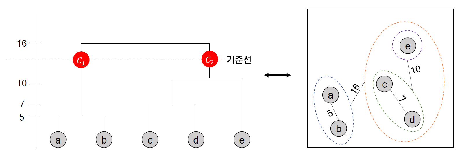
* 덴드로그램의 현실
- 덴드로그램은 샘플 수가 많은 경우에는 해석이 불가능할 정도로 복잡해진다는 문제가 있다.

// 100개 미만은 군집화가 필요 없을 것인데.. 샘플수가 7천개나되는 데이터가 위와 같다.
* 계층 군집화의 장단점
- 장점 (1) 덴드로그램을 이용한 군집화 과정 확인 가능
// 실제로는 데이터가 크면 그것도 쉽지가 않다는 의미이다.
- 장점 (2) 거리 / 유사도 행렬만 있으면 군집화 가능
- 장점 (3) 다양한 거리 척도 활용 가능
- 장점 (4) 수행할 때마다 같은 결과를 냄 (임의성 존재 x)
- 단점 (1) 상대적으로 많은 계산량 O(n^3)
// 데이터가 크면 그만큼 시간이 오래 걸린다.
- 단점 (2) 군집 개수 설정에 대한 제약 존재
* sklearn.cluster.AgglomerativeClustering
- 주요 입력
. n_clusters : 군집 개수
. affinity : 거리 척도 {"Euclidean", "manhattan", "cosine", "precomputed"}
.. linkage 가 ward 로 입력되면 "Euclidean"만 사용 가능함
// 그 이유는 각 군집마다 중심점을 필요로 하기 때문에 euclidean 은 중심을 표현하기 때문에 그런 것이다.
.. "precomputed" 는 거리 혹은 유사도 행렬을 입력으로 하는 경우에 설정하는 값
// 데이터를 바탕으로 거리를 계산하는 것이 아니다.
// 생각보다 많이 쓰는 키워드 설정이다.
. linkage : 군집 간 거리 { "ward", "complete", "average", "single"}
.. complete: 최장 연결법
.. average : 평균 연결법
.. single : 최단 연결법
- 주요 메서드
. fix(x) : 데이터 x에 대한 군집화 모델 학습
. fit_predict(x): 데이터 x 에 대한 군집화 모델 학습 및 라벨 반환
- 주요 속성
. labels_: fitting한 데이터에 있는 샘플들이 속한 군집 정보 (ndarray)
// skearn.cluster.AgglomeratevieClustering Documentation
scikit-learn.org/stable/modules/generated/sklearn.cluster.AgglomerativeClustering.html
class sklearn.cluster.AgglomerativeClustering(n_clusters=2, *, affinity='euclidean', memory=None, connectivity=None, compute_full_tree='auto', linkage='ward', distance_threshold=None)Agglomerative Clustering
Recursively merges the pair of clusters that minimally increases a given linkage distance.
Read more in the User Guide.
Parameters
n_clustersint or None, default=2
The number of clusters to find. It must be None if distance_threshold is not None.
affinitystr or callable, default=’euclidean’
Metric used to compute the linkage. Can be “euclidean”, “l1”, “l2”, “manhattan”, “cosine”, or “precomputed”. If linkage is “ward”, only “euclidean” is accepted. If “precomputed”, a distance matrix (instead of a similarity matrix) is needed as input for the fit method.
memorystr or object with the joblib.Memory interface, default=None
Used to cache the output of the computation of the tree. By default, no caching is done. If a string is given, it is the path to the caching directory.
connectivityarray-like or callable, default=None
Connectivity matrix. Defines for each sample the neighboring samples following a given structure of the data. This can be a connectivity matrix itself or a callable that transforms the data into a connectivity matrix, such as derived from kneighbors_graph. Default is None, i.e, the hierarchical clustering algorithm is unstructured.
compute_full_tree‘auto’ or bool, default=’auto’
Stop early the construction of the tree at n_clusters. This is useful to decrease computation time if the number of clusters is not small compared to the number of samples. This option is useful only when specifying a connectivity matrix. Note also that when varying the number of clusters and using caching, it may be advantageous to compute the full tree. It must be True if distance_threshold is not None. By default compute_full_tree is “auto”, which is equivalent to True when distance_threshold is not None or that n_clusters is inferior to the maximum between 100 or 0.02 * n_samples. Otherwise, “auto” is equivalent to False.
linkage{“ward”, “complete”, “average”, “single”}, default=”ward”
Which linkage criterion to use. The linkage criterion determines which distance to use between sets of observation. The algorithm will merge the pairs of cluster that minimize this criterion.
-
ward minimizes the variance of the clusters being merged.
-
average uses the average of the distances of each observation of the two sets.
-
complete or maximum linkage uses the maximum distances between all observations of the two sets.
-
single uses the minimum of the distances between all observations of the two sets.
New in version 0.20: Added the ‘single’ option
distance_thresholdfloat, default=None
The linkage distance threshold above which, clusters will not be merged. If not None, n_clusters must be None and compute_full_tree must be True.
New in version 0.21.
Attributes
n_clusters_int
The number of clusters found by the algorithm. If distance_threshold=None, it will be equal to the given n_clusters.
labels_ndarray of shape (n_samples)
cluster labels for each point
n_leaves_int
Number of leaves in the hierarchical tree.
n_connected_components_int
The estimated number of connected components in the graph.
New in version 0.21: n_connected_components_ was added to replace n_components_.
children_array-like of shape (n_samples-1, 2)
The children of each non-leaf node. Values less than n_samples correspond to leaves of the tree which are the original samples. A node i greater than or equal to n_samples is a non-leaf node and has children children_[i - n_samples]. Alternatively at the i-th iteration, children[i][0] and children[i][1] are merged to form node n_samples + i
Methods
|
fit(X[, y]) |
Fit the hierarchical clustering from features, or distance matrix. |
|
fit_predict(X[, y]) |
Fit the hierarchical clustering from features or distance matrix, and return cluster labels. |
|
get_params([deep]) |
Get parameters for this estimator. |
|
set_params(**params) |
Set the parameters of this estimator. |
[파이썬을 활용한 데이터 전처리 Level UP-Comment]
- 머신러닝에 대해서는 추후에 머신러닝 프로젝트에서 다룰 것이라서 간단하게 코멘트만 하고 넘어 갔는데.. 군집화 범주형에 대해서 처리를 할때 필요한 것이긴 하지만.. 어렵다. ㅠ.ㅠ.. 역시 이론만 들어서는 너무 어렵군.
파이썬을 활용한 데이터 전처리 Level UP 올인원 패키지 Online. | 패스트캠퍼스
데이터 분석에 필요한 기초 전처리부터, 데이터의 품질 및 머신러닝 성능 향상을 위한 고급 스킬까지 완전 정복하는 데이터 전처리 트레이닝 온라인 강의입니다.
www.fastcampus.co.kr
'Programming > Python' 카테고리의 다른 글
| [패스트캠퍼스 수강 후기] 데이터전처리 100% 환급 챌린지 17회차 미션 (0) | 2020.11.18 |
|---|---|
| [패스트캠퍼스 수강 후기] 데이터전처리 100% 환급 챌린지 16회차 미션 (0) | 2020.11.17 |
| [패스트캠퍼스 수강 후기] 데이터전처리 100% 환급 챌린지 14회차 미션 (2) | 2020.11.15 |
| [패스트캠퍼스 수강 후기] 데이터전처리 100% 환급 챌린지 13회차 미션 (2) | 2020.11.14 |
| [패스트캠퍼스 수강 후기] 데이터전처리 100% 환급 챌린지 12회차 미션 (2) | 2020.11.13 |