[패스트캠퍼스 수강 후기] 데이터전처리 100% 환급 챌린지 14회차 미션 Programming/Python2020. 11. 15. 11:43
[파이썬을 활용한 데이터 전처리 Level UP- 14 회차 미션 시작]
* 복습
- 쌍체표본 t- 검정, 독립 표본 t- 검정, 단일 표본 t- 검정의 각각의 의미와 p-value를 통한 검증에 대한 결과에 대한 해석을 엿볼 수 있었다. 다만 아직까지는 좀 더 많은 실습과 경험이 필요한 것 같다.
[02. Part 2) 탐색적 데이터 분석 Chapter 10. 둘 사이에는 무슨 관계가 있을까 - 가설 검정과 변수 간 관계 분석 - 04. 일원분산분석]

// 독립검정 t-검정에 대해서 배워볼 수 있었다.
* 일원분산분석 개요
- 목적 : 셋 이상의 그룹 간 차이가 존재하는지를 확인하기 위한 가설 검정 방법이다.
- 영 가설과 대립 가설

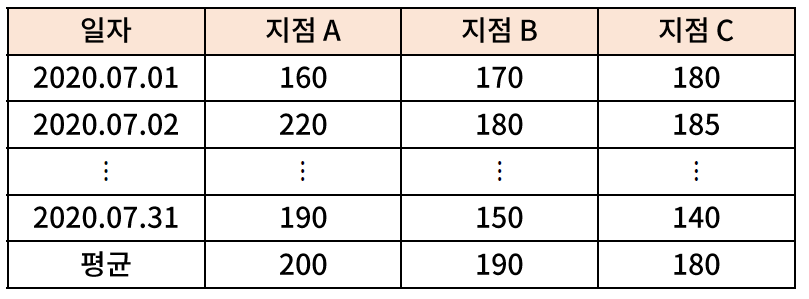
- 가설 수립 예시 : 2020년 7월 한 달 간 지점 A, B, C 의 일별 판매량이 아래와 같다면, 지점별 7월 판매량 간 유의미한 차이가 있는가? 또한, 어느 지점 간에는 유의미한 판매량 차이가 존재하지 않는가?
* 독립 표본 검정 t 검정을 사용하면 안되는 이유
- 일원분산분석은 독립 표본 t검정을 여러번 사용한 것과 같은 결과를 낼 것처럼 보인다.

- 독립 표본 t 검정에서 하나 이상의 영 가설이 기각되면, 자연스레 일원분산 분석의 영가설 역시 기각되므로, 기각된 원인까지 알 수 있으므로 일원분산분석이 필요하지 않아 보일 수 있다.
// p-value 를 기각했을때도 오류가 발생할 수가 있다.
- 그러나 독립 표본 t 검정을 여러번 했을때, 아무리 높은 p-value 가 나오더라도 그 신뢰성에 문제가 생길 수 있어, 일원분산분석이 필요하다.
. 각 가설의 p-value 가 0.95 이고, 그룹의 개수가 k일때 모든 영가설이 참일 확률 : 0.95^k
// k 승이 맞다는것은 점점 확률이 점점 떨어진다는 것을 의미하는 것이다.
. 그룹의 개수가 3개만 되어도 그 확률이 0.857로 크게 감소하며, 그룹의 개수가 14개가 되면 그 확률이 0.5 미만으로 떨어진다.
* 일원분산분석의 선행 분석
// 독립 표본 t-검정과 비슷한 점이 있다.
- 독립성 : 모든 그룹은 서로 독립적이어야 한다.
- 정규성 : 모든 그룹의 데이터는 정규분포를 따라야 한다.
. 그렇지 않으면 비모수적인 방법인 Kriskal-Wallis H Test 를 수행해야 한다.
- 등분산성 : 모든 그룹에 데이터에 대한 분산이 같아야 한다.
. 그렇지 않으면 비모수적인 방법인 Kruskal-Wallis H Test 를 수행해야 한다.
* 일원분산분석의 통계량
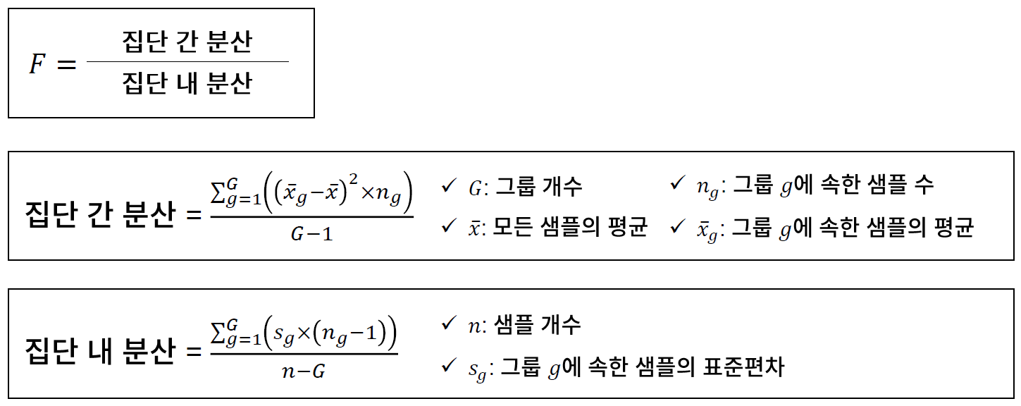
// F 통계량
// 집단 간의 차이가 크면 클 수록 값이 F 통계량이 커진다.
* 사후분석 : Tukey HSD test
- Tukey HSD (honestly significant difference) test 는 일원분산분석에서 두 그룹 a와 b 간 차이가 유의한 지 파악하는 사후 분석 방법이다.
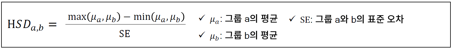
- 만약, HSD a,b 가 유의 수준보다 크면 두 차이가 유의하다고 간주
// 사후 분석을 통해서 어떤 그룹의 차이를 알 수 있다.
* 파이썬을 이용한 일원분산분석

// kstest 를 통해서 먼저 정규성을 검증을 먼저 한다.
// 사후분석과 일원분산분석은 구조가 다르다. scipy에는 없기때문에 다른 module에서 불러옴
// scipy.stas.f_oneway documentation
docs.scipy.org/doc/scipy/reference/generated/scipy.stats.f_oneway.html
scipy.stats.f_oneway(*args, axis=0)
Perform one-way ANOVA.
The one-way ANOVA tests the null hypothesis that two or more groups have the same population mean. The test is applied to samples from two or more groups, possibly with differing sizes.
Parameters
sample1, sample2, …array_like
The sample measurements for each group. There must be at least two arguments. If the arrays are multidimensional, then all the dimensions of the array must be the same except for axis.
axisint, optional
Axis of the input arrays along which the test is applied. Default is 0.
Returns
statisticfloat
The computed F statistic of the test.
pvaluefloat
The associated p-value from the F distribution.
WarnsF_onewayConstantInputWarning
Raised if each of the input arrays is constant array. In this case the F statistic is either infinite or isn’t defined, so np.inf or np.nan is returned.
F_onewayBadInputSizesWarning
Raised if the length of any input array is 0, or if all the input arrays have length 1. np.nan is returned for the F statistic and the p-value in these cases.
// statsmodels.stats.multicomp.pairwise_tukeyhsd documentation
www.statsmodels.org/stable/generated/statsmodels.stats.multicomp.pairwise_tukeyhsd.html
statsmodels.stats.multicomp.pairwise_tukeyhsd(endog, groups, alpha=0.05)
Calculate all pairwise comparisons with TukeyHSD confidence intervals
Parameters
response variable
groupsndarray, 1d
array with groups, can be string or integers
alphafloat
significance level for the test
Returns
resultsTukeyHSDResults instance
A results class containing relevant data and some post-hoc calculations, including adjusted p-value
* 실습
// A, B, C 2차원 배열..ndarray

// C가 평균이 확실히 크다라고 생각 할 수 있고, 이 정도의 차이이면 아노바 검증을 할 필요가 없다.
// A, B 는 검증을 해야봐야 한다.
// 일원분산분석 수행 : p-value 가 거의 0에 수렴 => A, B, C의 평균은 유의한 차이가 존재하는지.
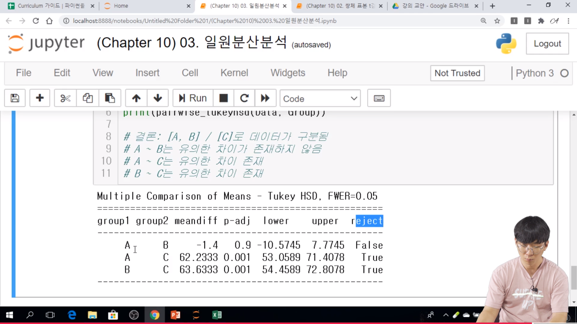
// False 는 둘의 차이가 없다라는 의미이다.
[02. Part 2) 탐색적 데이터 분석 Chapter 10. 둘 사이에는 무슨 관계가 있을까 - 가설 검정과 변수 간 관계 분석 - 04. 상관 분석]

// 연속 변수를 보는 상관분석과, 범주형 변수에서 볼수 있는 카이제곱검정이라고 보면 된다.
* 상관분석 개요
- 목적 : 두 연속형 변수 간에 어떠한 선형 관계를 가지는지 파악
// x가 증가하면 y가 증가한다, 감소하면 감소한다가.. 선형 관계이다.
- 영 가설과 대립 가설
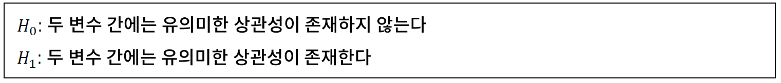
- 시각화 방법 : 산점도 (scatter plot)
* 피어슨 상관 계수
- 두 변수 모두 연속형 변수일 때 사용하는 상관 계수로 x와 y에 대한 상관 계수 p x,y 는 다음과 같이 정의된다.

- 상관 계수가 1에 가까울수록 양의 상관관계가 강하다고 하며, -1에 가까울수록 음의 상관관계가 강하다고 한다. 또한, 0에 가까울수록 상관관계가 약하다고 한다.
* 피어슨 상관 계수

// 선형관계라는 것은 선으로 이어져 있는 것을 확인하는 것이라고도 볼 수 있다.
// 선으로 볼 수 없는 것들은 피어슨 상관관계로 볼 수 없다.
* 스피어만 상관 계수
- 두 변수의 순위 사이의 단조 관련성을 측정하는 상관 계수로 x와 y에 대한 스피어만 상관 계수 S x,y 는 다음과 같이 정의된다.

* 파이썬을 이용한 상관분석

// 피어슨 상관계수에서 x, y 의 순서는 그렇게 중요하지 않다.
// scipy.stats.pearsonr documentation
docs.scipy.org/doc/scipy/reference/generated/scipy.stats.pearsonr.html
scipy.stats.pearsonr(x, y)
Pearson correlation coefficient and p-value for testing non-correlation.
The Pearson correlation coefficient [1] measures the linear relationship between two datasets. The calculation of the p-value relies on the assumption that each dataset is normally distributed. (See Kowalski [3] for a discussion of the effects of non-normality of the input on the distribution of the correlation coefficient.) Like other correlation coefficients, this one varies between -1 and +1 with 0 implying no correlation. Correlations of -1 or +1 imply an exact linear relationship. Positive correlations imply that as x increases, so does y. Negative correlations imply that as x increases, y decreases.
The p-value roughly indicates the probability of an uncorrelated system producing datasets that have a Pearson correlation at least as extreme as the one computed from these datasets.
Parameters
x(N,) array_like
Input array.
y(N,) array_like
Input array.
Returns
rfloat
Pearson’s correlation coefficient.
p-valuefloat
Two-tailed p-value.
Warns
PearsonRConstantInputWarning
Raised if an input is a constant array. The correlation coefficient is not defined in this case, so np.nan is returned.
PearsonRNearConstantInputWarning
Raised if an input is “nearly” constant. The array x is considered nearly constant if norm(x - mean(x)) < 1e-13 * abs(mean(x)). Numerical errors in the calculation x - mean(x) in this case might result in an inaccurate calculation of r.
// pandas.DataFrame.corr documentation
pandas.pydata.org/pandas-docs/stable/reference/api/pandas.DataFrame.corr.html
DataFrame.corr(method='pearson', min_periods=1)
Compute pairwise correlation of columns, excluding NA/null values.
Parameters
method{‘pearson’, ‘kendall’, ‘spearman’} or callable
Method of correlation:
pearson : standard correlation coefficient
kendall : Kendall Tau correlation coefficient
spearman : Spearman rank correlation
- callable: callable with input two 1d ndarrays
and returning a float. Note that the returned matrix from corr will have 1 along the diagonals and will be symmetric regardless of the callable’s behavior.
New in version 0.24.0.
min_periodsint, optional
Minimum number of observations required per pair of columns to have a valid result. Currently only available for Pearson and Spearman correlation.
Returns
DataFrame
Correlation matrix.
* 실습

// 처음은 양의 값.. 같이 증가 한다는 의미이다.
[02. Part 2) 탐색적 데이터 분석 Chapter 10. 둘 사이에는 무슨 관계가 있을까 - 가설 검정과 변수 간 관계 분석 - 04. 카이제곱검정]
* 카이제곱 검정 개요
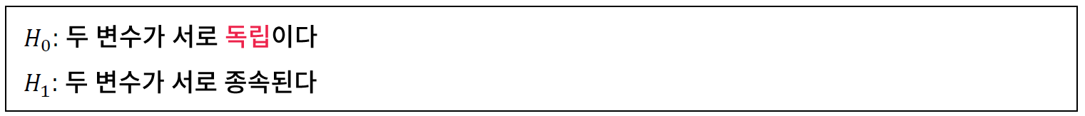
- 목적 : 두 점부형 변수가 서로 독립적인지 검정
- 영 가설과 대립 가설
- 시각화 방법 : 교차 테이블
* 교차 테이블과 기대값
- 교차 테이블(contingency table) 은 두 변수가 취할 수 있는 값의 조합의 출현 빈도를 나타낸다.
- 예시 : 성별에 따른 강의 만족도 (카테고리 수 = 2 x 3 = 6)
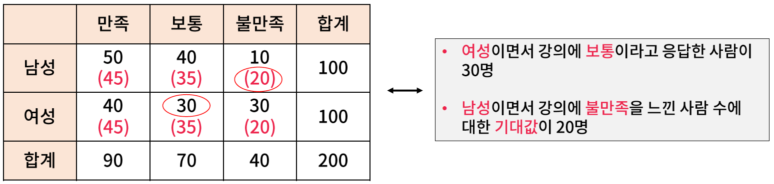
// 빨간색은 기대값.

* 카이제곱 통계량
- 카이제곱 검정에 사용하는 카이제곱 통계량은 기대값과 실제값의 차이를 바탕으로 정의된다.

- 기대값과 실제값의 차이가 클수록 통계량이 커지며, 통계량이 커질수록 영 가설이 기각될 가능성이 높아진다. (즉, p-value 가 감소)
* 파이썬을 이용한 카이제곱 검정

// 시리즈이면서 범주형
// dof 자유도, expected 기대값
// pandas.crosstab documenation
pandas.pydata.org/pandas-docs/stable/reference/api/pandas.crosstab.html
pandas.crosstab(index, columns, values=None, rownames=None, colnames=None, aggfunc=None, margins=False, margins_name='All', dropna=True, normalize=False)
Compute a simple cross tabulation of two (or more) factors. By default computes a frequency table of the factors unless an array of values and an aggregation function are passed.
Parameters
indexarray-like, Series, or list of arrays/Series
Values to group by in the rows.
columnsarray-like, Series, or list of arrays/Series
Values to group by in the columns.
valuesarray-like, optional
Array of values to aggregate according to the factors. Requires aggfunc be specified.
rownamessequence, default None
If passed, must match number of row arrays passed.
colnamessequence, default None
If passed, must match number of column arrays passed.
aggfuncfunction, optional
If specified, requires values be specified as well.
marginsbool, default False
Add row/column margins (subtotals).
margins_namestr, default ‘All’
Name of the row/column that will contain the totals when margins is True.
dropnabool, default True
Do not include columns whose entries are all NaN.
normalizebool, {‘all’, ‘index’, ‘columns’}, or {0,1}, default False
Normalize by dividing all values by the sum of values.
If passed ‘all’ or True, will normalize over all values.
If passed ‘index’ will normalize over each row.
If passed ‘columns’ will normalize over each column.
If margins is True, will also normalize margin values.
Returns
DataFrame
Cross tabulation of the data.
// scipy.stats.chi2_contingency documentation
docs.scipy.org/doc/scipy/reference/generated/scipy.stats.chi2_contingency.html
scipy.stats.chi2_contingency(observed, correction=True, lambda_=None)
Chi-square test of independence of variables in a contingency table.
This function computes the chi-square statistic and p-value for the hypothesis test of independence of the observed frequencies in the contingency table [1] observed. The expected frequencies are computed based on the marginal sums under the assumption of independence; see scipy.stats.contingency.expected_freq. The number of degrees of freedom is (expressed using numpy functions and attributes):
dof = observed.size - sum(observed.shape) + observed.ndim - 1
Parameters
observedarray_like
The contingency table. The table contains the observed frequencies (i.e. number of occurrences) in each category. In the two-dimensional case, the table is often described as an “R x C table”.
correctionbool, optional
If True, and the degrees of freedom is 1, apply Yates’ correction for continuity. The effect of the correction is to adjust each observed value by 0.5 towards the corresponding expected value.
lambda_float or str, optional.
By default, the statistic computed in this test is Pearson’s chi-squared statistic [2]. lambda_ allows a statistic from the Cressie-Read power divergence family [3] to be used instead. See power_divergence for details.
Returns
chi2float
The test statistic.
pfloat
The p-value of the test
dofint
Degrees of freedom
expectedndarray, same shape as observed
The expected frequencies, based on the marginal sums of the table.
* 실습
// pvalue 0.0018 로 두 변수 간 독립이 아님을 확인할 수 있다. 서로 종속적이다라고 확인할 수 있다.
[파이썬을 활용한 데이터 전처리 Level UP-Comment]
- 일원분석.. 상관분석과 카이제곱 검정에서 대해서 알아봤다. 어렵다. 이론적인 배경 설명위주로 해서 그런지 넘 어렵게 느껴진다. ㅠ.ㅠ
파이썬을 활용한 데이터 전처리 Level UP 올인원 패키지 Online. | 패스트캠퍼스
데이터 분석에 필요한 기초 전처리부터, 데이터의 품질 및 머신러닝 성능 향상을 위한 고급 스킬까지 완전 정복하는 데이터 전처리 트레이닝 온라인 강의입니다.
www.fastcampus.co.kr
'Programming > Python' 카테고리의 다른 글
| [패스트캠퍼스 수강 후기] 데이터전처리 100% 환급 챌린지 16회차 미션 (0) | 2020.11.17 |
|---|---|
| [패스트캠퍼스 수강 후기] 데이터전처리 100% 환급 챌린지 15회차 미션 (2) | 2020.11.16 |
| [패스트캠퍼스 수강 후기] 데이터전처리 100% 환급 챌린지 13회차 미션 (2) | 2020.11.14 |
| [패스트캠퍼스 수강 후기] 데이터전처리 100% 환급 챌린지 12회차 미션 (2) | 2020.11.13 |
| [패스트캠퍼스 수강 후기] 데이터전처리 100% 환급 챌린지 11회차 미션 (2) | 2020.11.12 |