The one-way ANOVA tests the null hypothesis that two or more groups have the same population mean. The test is applied to samples from two or more groups, possibly with differing sizes.
Parameters
sample1, sample2, …array_like
The sample measurements for each group. There must be at least two arguments. If the arrays are multidimensional, then all the dimensions of the array must be the same except for axis.
axisint, optional
Axis of the input arrays along which the test is applied. Default is 0.
Returns
statisticfloat
The computed F statistic of the test.
pvaluefloat
The associated p-value from the F distribution.
WarnsF_onewayConstantInputWarning
Raised if each of the input arrays is constant array. In this case the F statistic is either infinite or isn’t defined, so np.inf or np.nan is returned.
F_onewayBadInputSizesWarning
Raised if the length of any input array is 0, or if all the input arrays have length 1. np.nan is returned for the F statistic and the p-value in these cases.
Pearson correlation coefficient and p-value for testing non-correlation.
The Pearson correlation coefficient [1] measures the linear relationship between two datasets. The calculation of the p-value relies on the assumption that each dataset is normally distributed. (See Kowalski [3] for a discussion of the effects of non-normality of the input on the distribution of the correlation coefficient.) Like other correlation coefficients, this one varies between -1 and +1 with 0 implying no correlation. Correlations of -1 or +1 imply an exact linear relationship. Positive correlations imply that as x increases, so does y. Negative correlations imply that as x increases, y decreases.
The p-value roughly indicates the probability of an uncorrelated system producing datasets that have a Pearson correlation at least as extreme as the one computed from these datasets.
Parameters
x(N,) array_like
Input array.
y(N,) array_like
Input array.
Returns
rfloat
Pearson’s correlation coefficient.
p-valuefloat
Two-tailed p-value.
Warns
PearsonRConstantInputWarning
Raised if an input is a constant array. The correlation coefficient is not defined in this case, so np.nan is returned.
PearsonRNearConstantInputWarning
Raised if an input is “nearly” constant. The array x is considered nearly constant if norm(x - mean(x)) < 1e-13 * abs(mean(x)). Numerical errors in the calculation x - mean(x) in this case might result in an inaccurate calculation of r.
Compute pairwise correlation of columns, excluding NA/null values.
Parameters
method{‘pearson’, ‘kendall’, ‘spearman’} or callable
Method of correlation:
pearson : standard correlation coefficient
kendall : Kendall Tau correlation coefficient
spearman : Spearman rank correlation
callable: callable with input two 1d ndarrays
and returning a float. Note that the returned matrix from corr will have 1 along the diagonals and will be symmetric regardless of the callable’s behavior.
New in version 0.24.0.
min_periodsint, optional
Minimum number of observations required per pair of columns to have a valid result. Currently only available for Pearson and Spearman correlation.
Returns
DataFrame
Correlation matrix.
* 실습
// 처음은 양의 값.. 같이 증가 한다는 의미이다.
[02. Part 2) 탐색적 데이터 분석 Chapter 10. 둘 사이에는 무슨 관계가 있을까 - 가설 검정과 변수 간 관계 분석 - 04. 카이제곱검정]
* 카이제곱 검정 개요
- 목적 : 두 점부형 변수가 서로 독립적인지 검정
- 영 가설과 대립 가설
- 시각화 방법 : 교차 테이블
* 교차 테이블과 기대값
- 교차 테이블(contingency table) 은 두 변수가 취할 수 있는 값의 조합의 출현 빈도를 나타낸다.
- 예시 : 성별에 따른 강의 만족도 (카테고리 수 = 2 x 3 = 6)
// 빨간색은 기대값.
* 카이제곱 통계량
- 카이제곱 검정에 사용하는 카이제곱 통계량은 기대값과 실제값의 차이를 바탕으로 정의된다.
- 기대값과 실제값의 차이가 클수록 통계량이 커지며, 통계량이 커질수록 영 가설이 기각될 가능성이 높아진다. (즉, p-value 가 감소)
Compute a simple cross tabulation of two (or more) factors. By default computes a frequency table of the factors unless an array of values and an aggregation function are passed.
Parameters
indexarray-like, Series, or list of arrays/Series
Values to group by in the rows.
columnsarray-like, Series, or list of arrays/Series
Values to group by in the columns.
valuesarray-like, optional
Array of values to aggregate according to the factors. Requires aggfunc be specified.
rownamessequence, default None
If passed, must match number of row arrays passed.
colnamessequence, default None
If passed, must match number of column arrays passed.
aggfuncfunction, optional
If specified, requires values be specified as well.
marginsbool, default False
Add row/column margins (subtotals).
margins_namestr, default ‘All’
Name of the row/column that will contain the totals when margins is True.
dropnabool, default True
Do not include columns whose entries are all NaN.
normalizebool, {‘all’, ‘index’, ‘columns’}, or {0,1}, default False
Normalize by dividing all values by the sum of values.
If passed ‘all’ orTrue, will normalize over all values.
If passed ‘index’ will normalize over each row.
If passed ‘columns’ will normalize over each column.
If margins isTrue, will also normalize margin values.
Chi-square test of independence of variables in a contingency table.
This function computes the chi-square statistic and p-value for the hypothesis test of independence of the observed frequencies in the contingency table [1] observed. The expected frequencies are computed based on the marginal sums under the assumption of independence; see scipy.stats.contingency.expected_freq. The number of degrees of freedom is (expressed using numpy functions and attributes):
The contingency table. The table contains the observed frequencies (i.e. number of occurrences) in each category. In the two-dimensional case, the table is often described as an “R x C table”.
correctionbool, optional
If True, and the degrees of freedom is 1, apply Yates’ correction for continuity. The effect of the correction is to adjust each observed value by 0.5 towards the corresponding expected value.
lambda_float or str, optional.
By default, the statistic computed in this test is Pearson’s chi-squared statistic [2]. lambda_ allows a statistic from the Cressie-Read power divergence family [3] to be used instead. See power_divergence for details.
Returns
chi2float
The test statistic.
pfloat
The p-value of the test
dofint
Degrees of freedom
expectedndarray, same shape as observed
The expected frequencies, based on the marginal sums of the table.
* 실습
// pvalue 0.0018 로 두 변수 간 독립이 아님을 확인할 수 있다. 서로 종속적이다라고 확인할 수 있다.
[파이썬을 활용한 데이터 전처리 Level UP-Comment] - 일원분석.. 상관분석과 카이제곱 검정에서 대해서 알아봤다. 어렵다. 이론적인 배경 설명위주로 해서 그런지 넘 어렵게 느껴진다. ㅠ.ㅠ
Performs the (one sample or two samples) Kolmogorov-Smirnov test for goodness of fit.
The one-sample test performs a test of the distribution F(x) of an observed random variable against a given distribution G(x). Under the null hypothesis, the two distributions are identical, F(x)=G(x). The alternative hypothesis can be either ‘two-sided’ (default), ‘less’ or ‘greater’. The KS test is only valid for continuous distributions. The two-sample test tests whether the two independent samples are drawn from the same continuous distribution.
Parameters
rvsstr, array_like, or callable
If an array, it should be a 1-D array of observations of random variables. If a callable, it should be a function to generate random variables; it is required to have a keyword argumentsize. If a string, it should be the name of a distribution inscipy.stats, which will be used to generate random variables.
cdfstr, array_like or callable
If array_like, it should be a 1-D array of observations of random variables, and the two-sample test is performed (and rvs must be array_like) If a callable, that callable is used to calculate the cdf. If a string, it should be the name of a distribution inscipy.stats, which will be used as the cdf function.
argstuple, sequence, optional
Distribution parameters, used ifrvsorcdfare strings or callables.
Nint, optional
Sample size ifrvsis string or callable. Default is 20.
Calculate the T-test for the mean of ONE group of scores.
This is a two-sided test for the null hypothesis that the expected value (mean) of a sample of independent observationsais equal to the given population mean,popmean.
Parameters
aarray_like
Sample observation.
popmeanfloat or array_like
Expected value in null hypothesis. If array_like, then it must have the same shape asaexcluding the axis dimension.
axisint or None, optional
Axis along which to compute test. If None, compute over the whole arraya.
The Wilcoxon signed-rank test tests the null hypothesis that two related paired samples come from the same distribution. In particular, it tests whether the distribution of the differences x - y is symmetric about zero. It is a non-parametric version of the paired T-test.
Parameters
xarray_like
Either the first set of measurements (in which caseyis the second set of measurements), or the differences between two sets of measurements (in which caseyis not to be specified.) Must be one-dimensional.
yarray_like, optional
Either the second set of measurements (ifxis the first set of measurements), or not specified (ifxis the differences between two sets of measurements.) Must be one-dimensional.
The following options are available (default is ‘wilcox’):
‘pratt’: Includes zero-differences in the ranking process, but drops the ranks of the zeros, see[4], (more conservative).
‘wilcox’: Discards all zero-differences, the default.
‘zsplit’: Includes zero-differences in the ranking process and split the zero rank between positive and negative ones.
correctionbool, optional
If True, apply continuity correction by adjusting the Wilcoxon rank statistic by 0.5 towards the mean value when computing the z-statistic if a normal approximation is used. Default is False.
The alternative hypothesis to be tested, see Notes. Default is “two-sided”.
mode{“auto”, “exact”, “approx”}
Method to calculate the p-value, see Notes. Default is “auto”.
Returns
statisticfloat
Ifalternativeis “two-sided”, the sum of the ranks of the differences above or below zero, whichever is smaller. Otherwise the sum of the ranks of the differences above zero.
pvaluefloat
The p-value for the test depending onalternativeandmode.
* 실습
// 0.0 으로 나왔기 때문에 0.05보다 낮아서 정규성을 띈다고 볼 수 있다.
// 단일 표본 t 검정 수행
// 0.05 미만이므로 영가설은 기각되고, 통계량이 음수이므로 data 평균이 163보다 작는 것을 알 수 있다.
[02. Part 2) 탐색적 데이터 분석Chapter 10. 둘 사이에는 무슨 관계가 있을까 - 가설 검정과 변수 간 관계 분석 - 02. 독립 표본 t 검정]
* 독립 표본 t - 검정 개요
- 목적 : 서로 다른 두 그룹의 데이터 평균 비교
// 단일 표본 t-검정 보다는 더 많이 쓰인다.
- 영 가설과 대립 가설
- 가설 수립 예시 : 2020년 7월 한 달 간 지점 A의 일별 판매량과 지점 B의 일별 판매량이 아래와 같다면, 지점 A와 지점 B의 7월 판매량 간 유의미한 차이가 있는가?
The Levene test tests the null hypothesis that all input samples are from populations with equal variances. Levene’s test is an alternative to Bartlett’s testbartlettin the case where there are significant deviations from normality.
Calculate the T-test for the means oftwo independentsamples of scores.
This is a two-sided test for the null hypothesis that 2 independent samples have identical average (expected) values. This test assumes that the populations have identical variances by default.
Parameters
a, barray_like
The arrays must have the same shape, except in the dimension corresponding toaxis(the first, by default).
axisint or None, optional
Axis along which to compute test. If None, compute over the whole arrays,a, andb.
equal_varbool, optional
If True (default), perform a standard independent 2 sample test that assumes equal population variances[1]. If False, perform Welch’s t-test, which does not assume equal population variance[2].
Defines the alternative hypothesis. The following options are available (default is None):
None: computes p-value half the size of the ‘two-sided’ p-value and a different U statistic. The default behavior is not the same as using ‘less’ or ‘greater’; it only exists for backward compatibility and is deprecated.
‘two-sided’
‘less’: one-sided
‘greater’: one-sided
Use of the None option is deprecated.
Returns
statisticfloat
The Mann-Whitney U statistic, equal to min(U for x, U for y) ifalternativeis equal to None (deprecated; exists for backward compatibility), and U for y otherwise.
pvaluefloat
p-value assuming an asymptotic normal distribution. One-sided or two-sided, depending on the choice ofalternative.
* 실습
// scipy 에서는 Series 보다는 ndarray 가 더 낮기 때문에 values 를 만들어서 들고 있다.
// 만약에 NaN 값이 있다면 float 형태로 나오기 때문에 수치에서 .0 으로 나온다면 NaN 이 있다는 것을 알 고 있어야 한다.
[02. Part 2) 탐색적 데이터 분석Chapter 10. 둘 사이에는 무슨 관계가 있을까 - 가설 검정과 변수 간 관계 분석 - 03. 쌍체 표본 t 검정]
numpy.percentile(a, q, axis=None, out=None, overwrite_input=False, interpolation='linear', keepdims=False)
Compute the q-th percentile of the data along the specified axis.
Returns the q-th percentile(s) of the array elements.
Parameters
aarray_like
Input array or object that can be converted to an array.
qarray_like of float
Percentile or sequence of percentiles to compute, which must be between 0 and 100 inclusive.
axis{int, tuple of int, None}, optional
Axis or axes along which the percentiles are computed. The default is to compute the percentile(s) along a flattened version of the array.
Changed in version 1.9.0:A tuple of axes is supported
outndarray, optional
Alternative output array in which to place the result. It must have the same shape and buffer length as the expected output, but the type (of the output) will be cast if necessary.
overwrite_inputbool, optional
If True, then allow the input arrayato be modified by intermediate calculations, to save memory. In this case, the contents of the inputaafter this function completes is undefined.
This optional parameter specifies the interpolation method to use when the desired percentile lies between two data pointsi<j:
‘linear’:i+(j-i)*fraction, wherefractionis the fractional part of the index surrounded byiandj.
‘lower’:i.
‘higher’:j.
‘nearest’:iorj, whichever is nearest.
‘midpoint’:(i+j)/2.
New in version 1.9.0.
keepdimsbool, optional
If this is set to True, the axes which are reduced are left in the result as dimensions with size one. With this option, the result will broadcast correctly against the original arraya.
New in version 1.9.0.
Returns
percentilescalar or ndarray
Ifqis a single percentile andaxis=None, then the result is a scalar. If multiple percentiles are given, first axis of the result corresponds to the percentiles. The other axes are the axes that remain after the reduction ofa. If the input contains integers or floats smaller thanfloat64, the output data-type isfloat64. Otherwise, the output data-type is the same as that of the input. Ifoutis specified, that array is returned instead.
numpy.quantile(a, q, axis=None, out=None, overwrite_input=False, interpolation='linear', keepdims=False)
Compute the q-th quantile of the data along the specified axis.
New in version 1.15.0.
Parameters
aarray_like
Input array or object that can be converted to an array.
qarray_like of float
Quantile or sequence of quantiles to compute, which must be between 0 and 1 inclusive.
axis{int, tuple of int, None}, optional
Axis or axes along which the quantiles are computed. The default is to compute the quantile(s) along a flattened version of the array.
outndarray, optional
Alternative output array in which to place the result. It must have the same shape and buffer length as the expected output, but the type (of the output) will be cast if necessary.
overwrite_inputbool, optional
If True, then allow the input arrayato be modified by intermediate calculations, to save memory. In this case, the contents of the inputaafter this function completes is undefined.
This optional parameter specifies the interpolation method to use when the desired quantile lies between two data pointsi<j:
linear:i+(j-i)*fraction, wherefractionis the fractional part of the index surrounded byiandj.
lower:i.
higher:j.
nearest:iorj, whichever is nearest.
midpoint:(i+j)/2.
keepdimsbool, optional
If this is set to True, the axes which are reduced are left in the result as dimensions with size one. With this option, the result will broadcast correctly against the original arraya.
Returns
quantilescalar or ndarray
Ifqis a single quantile andaxis=None, then the result is a scalar. If multiple quantiles are given, first axis of the result corresponds to the quantiles. The other axes are the axes that remain after the reduction ofa. If the input contains integers or floats smaller thanfloat64, the output data-type isfloat64. Otherwise, the output data-type is the same as that of the input. Ifoutis specified, that array is returned instead.
Input array or object that can be converted to an array.
axis{int, sequence of int, None}, optional
Axis or axes along which the medians are computed. The default is to compute the median along a flattened version of the array. A sequence of axes is supported since version 1.9.0.
outndarray, optional
Alternative output array in which to place the result. It must have the same shape and buffer length as the expected output, but the type (of the output) will be cast if necessary.
overwrite_inputbool, optional
If True, then allow use of memory of input arrayafor calculations. The input array will be modified by the call tomedian. This will save memory when you do not need to preserve the contents of the input array. Treat the input as undefined, but it will probably be fully or partially sorted. Default is False. Ifoverwrite_inputisTrueandais not already anndarray, an error will be raised.
keepdimsbool, optional
If this is set to True, the axes which are reduced are left in the result as dimensions with size one. With this option, the result will broadcast correctly against the originalarr.
New in version 1.9.0.
Returns
medianndarray
A new array holding the result. If the input contains integers or floats smaller thanfloat64, then the output data-type isnp.float64. Otherwise, the data-type of the output is the same as that of the input. Ifoutis specified, that array is returned instead.
* 실습
// 10% 값
* 왜도
- 왜도 (skewness) : 분포의 비대칭도를 나타내는 통계량
- 왜도가 음수면 오른쪾으로 치우친 것을 의미하며, 양수면 왼쪽으로 치우침을 의미한다.
// 0 일때는 정규분포형태라고 볼 수 있다.
- 일반적으로 왜도의 절대값이 1.5 이상이면 치우쳤다고 본다.
* 첨도
- 첨도 (kurtosis) : 데이터의 분포가 얼마나 뾰족한지를 의미한다. 즉, 첨도가 높을수록 이 변수가 좁은 범위에 많은 값들이 몰려있다고 할 수 있다.
For normally distributed data, the skewness should be about zero. For unimodal continuous distributions, a skewness value greater than zero means that there is more weight in the right tail of the distribution. The functionskewtestcan be used to determine if the skewness value is close enough to zero, statistically speaking.
Parameters
andarray
Input array.
axisint or None, optional
Axis along which skewness is calculated. Default is 0. If None, compute over the whole arraya.
biasbool, optional
If False, then the calculations are corrected for statistical bias.
Compute the kurtosis (Fisher or Pearson) of a dataset.
Kurtosis is the fourth central moment divided by the square of the variance. If Fisher’s definition is used, then 3.0 is subtracted from the result to give 0.0 for a normal distribution.
If bias is False then the kurtosis is calculated using k statistics to eliminate bias coming from biased moment estimators
Usekurtosistestto see if result is close enough to normal.
Parameters
aarray
Data for which the kurtosis is calculated.
axisint or None, optional
Axis along which the kurtosis is calculated. Default is 0. If None, compute over the whole arraya.
fisherbool, optional
If True, Fisher’s definition is used (normal ==> 0.0). If False, Pearson’s definition is used (normal ==> 3.0).
biasbool, optional
If False, then the calculations are corrected for statistical bias.
Defines how to handle when input contains nan. ‘propagate’ returns nan, ‘raise’ throws an error, ‘omit’ performs the calculations ignoring nan values. Default is ‘propagate’.
Returns
kurtosisarray
The kurtosis of values along an axis. If all values are equal, return -3 for Fisher’s definition and 0 for Pearson’s definition.
Return unbiased kurtosis over requested axis using Fisher’s definition of kurtosis (kurtosis of normal == 0.0). Normalized by N-1
Parameters: axis:{index (0)}
skipna: boolean, default True
level: int or level name, default None
numeric_only: boolean, default None
Returns: kurt:scalar or Series (if level specified)
* 실습
[02. Part 2) 탐색적 데이터 분석Chapter 09. 변수가 어떻게 생겼나 - 기초 통계 분석 - 05. 머신러닝에서의 기초 통계 분석]
* 변수 분포 문제 확인
- 머신러닝에서 각 변수를 이해하고, 특별한 분포 문제가 없는지 확인하기 위해 기초 통계 분석을 수행한다.
// 평균과 범위로 특징과 스케일링을 알 수 있다. 다시 말해서, 스케일의 편차를 줄인다고 보면 된다.
// 사분위는 이상치 제거를 볼 수가 있다.
// 왜도 같으면.. 1.5보다 크거나 작거나로 치우치는지를 확인해 볼수가 있다... 치우치거나 몰려 있게 되면 정규화를 통해 정의 할 수 있다.
[02. Part 2) 탐색적 데이터 분석Chapter 10. 둘 사이에는 무슨 관계가 있을까 - 가설 검정과 변수 간 관계 분석 - 01. 영가설과 대립가설, p-value]
* 통계적 가설 검정 개요
- 갖고 있는 샘플을 가지고 모집단의 특성에 대한 가설에 대한 통계적 유의성을 검정하는 일련의 과정
. 수집한 데이터는 매우 특별한 경우를 제외하고는 전부 샘플이며, 모집단은 정확히 알 수 없는 경우가 더 많다.
// 모집단을 정확히 알 수는 없다. 예를 들어 대한민국 남성의 모든 키를 알 수는 없고, 단지 수집한 자료를 가지고 활용할 것이다.
// 보통은 모집단을 알 수 없는 경우가 대부분이다.
. 통계적 유의성 : 어떤 실험 결과 (데이터)가 확률적으로 봐서 단순한 우연이 아니라고 판단될 정도로 의미가 있다.
- 통계적 가설 검정 과정은 다음과 같이 5단계로 구성된다.
* 영 가설과 대립 가설
- 영 가설 (null hypothesis)와 대립 가설(alternative hypothesis)로 구분하여, 가설을 수립해야 한다.
// 영 가설 -> 귀무가설
// 대립 가설 -> 우리가 알고 싶은 대상에 대한 가설
// 영 가설 -> 범죄자는 무죄이다.
// 대립 가설에서는 죄를 찾기 위해서 증거를 수집한다는 예로 들어서 생각해 볼 수 있다.
// 대립 가설 (H 알파..A 가 아니라)
// 양측 검정 -> 키가 크거나 작아도 되므로, 양측 검정
// 단측 검정 -> 성인 남성의 키가 크다라는 검을 검정한다는 의미로 생각하면 된다.
* 오류의 구분
- 가설 검정에서 발생하는 오류는 참을 거짓이라 하는 제 1종 오류 (type 1 Error)와 거짓을 참이라 하는 제 2종 오류로 구분된다.
// 샘플을 가지고 검증하기 때문에 오류가 반드시 난다고 생각하면 된다.
* 유의 확률, p-value
- 유의 확률 p-value : 영 가설이 맞다고 가정할 때 얻은 결과와 다른 결과가 관측될 확률로, 그 값이 작을수록 영 가설을 기각할 근거가 된다.
// 유의 확률, 영 가설, p-value 만 알아도 통계측에서는 90%이상 이해했다고 보면 된다.
- 보통, p-value 가 0.05 혹은 0.01 미만이면 영 가설을 기각한다.
// 영 가설을 기각한다고 해서 반드시 대립 가설이 참인것은 아니다. 새로운 검증을 해봐야 한다.
* 유의 확률, p-value (예시1)
- 영 가설 : 대한민국 성인 남성의 키는 160 cm 일 것이다.
- 대립 가설 : 대한민국 성인 남성의 키는 160 cm 이상일 것이다.
- 관측한 대한민국 성인 남성의 키의 평균은 175 cm, 표준편차는 1cm 이다.
* 유의 확률, p-value (예시2)
- 영 가설 : 대란민국 성인 남성의 키는 여성의 키와 같을 것이다.
- 대립 가설 : 대한민국 성인 남성의 키는 여성의 키보다 작다.
[파이썬을 활용한 데이터 전처리 Level UP-Comment] - 영가설, 대립가설, p-value 에 대해서 배웠다. p-value
- p-value
The p-value is about the strength of a hypothesis. We build hypothesis based on some statistical model and compare the model's validity using p-value. One way to get the p-value is by using T-test.
This is a two-sided test for the null hypothesis that the expected value (mean) of a sample of independent observations ‘a’ is equal to the given population mean,popmean. Let us consider the following example.
Compute the arithmetic mean along the specified axis.
Returns the average of the array elements. The average is taken over the flattened array by default, otherwise over the specified axis.float64intermediate and return values are used for integer inputs.
Parameters
a array_like
Array containing numbers whose mean is desired. Ifais not an array, a conversion is attempted.
axis None or int or tuple of ints, optional
Axis or axes along which the means are computed. The default is to compute the mean of the flattened array.
New in version 1.7.0.
If this is a tuple of ints, a mean is performed over multiple axes, instead of a single axis or all the axes as before.
dtype data-type, optional
Type to use in computing the mean. For integer inputs, the default isfloat64; for floating point inputs, it is the same as the input dtype.
out ndarray, optional
Alternate output array in which to place the result. The default isNone; if provided, it must have the same shape as the expected output, but the type will be cast if necessary. Seeufuncs-output-typefor more details.
keepdims bool, optional
If this is set to True, the axes which are reduced are left in the result as dimensions with size one. With this option, the result will broadcast correctly against the input array.
If the default value is passed, thenkeepdimswill not be passed through to themeanmethod of sub-classes ofndarray, however any non-default value will be. If the sub-class’ method does not implementkeepdimsany exceptions will be raised.
Returns
m ndarray, see dtype parameter above
Ifout=None, returns a new array containing the mean values, otherwise a reference to the output array is returned.
Calculate the harmonic mean along the specified axis.
That is: n / (1/x1 + 1/x2 + … + 1/xn)
Parameters
a array_like
Input array, masked array or object that can be converted to an array.
axis int or None, optional
Axis along which the harmonic mean is computed. Default is 0. If None, compute over the whole arraya.
dtype dtype, optional
Type of the returned array and of the accumulator in which the elements are summed. Ifdtypeis not specified, it defaults to the dtype ofa, unlessahas an integerdtypewith a precision less than that of the default platform integer. In that case, the default platform integer is used.
Return mean of array after trimming distribution from both tails.
Ifproportiontocut= 0.1, slices off ‘leftmost’ and ‘rightmost’ 10% of scores. The input is sorted before slicing. Slices off less if proportion results in a non-integer slice index (i.e., conservatively slices offproportiontocut).
Parameters
a array_like
Input array.
proportiontocut float
Fraction to cut off of both tails of the distribution.
axis int or None, optional
Axis along which the trimmed means are computed. Default is 0. If None, compute over the whole arraya.
Returns
trim_mean ndarray
Mean of trimmed array.
* 실습
// 100명의 소득 기준으로 해야하지, 1명의 값 10억원으로 갑자기 뛰면 평균 자체가 우리가 생각하는 평균에 비해서 다르게 나온다.
// trim_mean(income, 0.2) # [20% ~ 80%] 으로 하면 원래 1명을 제외한 기대값으로 나올 수가 있다.
* 최빈값
- 한 변수가 가장 많이 취한 값을 의미하며, 범주형 변수에 대해서만 적용한다.
- 파이썬을 이용한 최빈값 계산
. scipy.stats.mode(x)
. Series.value_counts().index[0] (주의 : 최빈값이 둘 이상이면 사용 불가)
// 값의 빈도에 따라서 정의 해주는 것이다.
* 실습
[02. Part 2) 탐색적 데이터 분석Chapter 09. 변수가 어떻게 생겼나 - 기초 통계 분석 - 03. 산포 통계량]
* 개요
- 산포란 데이터가 얼마나 퍼져있는지를 의미한다.
- 즉, 산포 통계량이란 데이터의 산포를 나타내는 통계량이라고 할 수 있다.
// 두 그래프 모두 확률 밀도 함수이다.
* 분산, 표준편차
- 편차 : 한 샘플이 평균으로부터 떨어진 거리, xi - u (xi : i 번째 관측치, u : 평균)
- 분산 : 편차의 제곱의 평균
-> 편차의 합은 항상 0이 되기 때문에, 제곱을 사용
-> 자유도가 0 (모분산)이면 n - 1 으로 나누지 않고, n 으로 나눔
- 표준편차 : 분산에 루트를 씌운 것
-> 분산에서 제곱의 영향을 없앤 지표
* 변동계수
- 분산과 표준 편차 모두 값의 스케일에 크게 영향을 받아, 상대적인 산포를 보여주는데 부적합하다.
Returns the variance of the array elements, a measure of the spread of a distribution. The variance is computed for the flattened array by default, otherwise over the specified axis.
Parameters
aarray_like
Array containing numbers whose variance is desired. Ifais not an array, a conversion is attempted.
axisNone or int or tuple of ints, optional
Axis or axes along which the variance is computed. The default is to compute the variance of the flattened array.
New in version 1.7.0.
If this is a tuple of ints, a variance is performed over multiple axes, instead of a single axis or all the axes as before.
dtypedata-type, optional
Type to use in computing the variance. For arrays of integer type the default isfloat64; for arrays of float types it is the same as the array type.
outndarray, optional
Alternate output array in which to place the result. It must have the same shape as the expected output, but the type is cast if necessary.
ddofint, optional
“Delta Degrees of Freedom”: the divisor used in the calculation isN-ddof, whereNrepresents the number of elements. By defaultddofis zero.
keepdimsbool, optional
If this is set to True, the axes which are reduced are left in the result as dimensions with size one. With this option, the result will broadcast correctly against the input array.
If the default value is passed, thenkeepdimswill not be passed through to thevarmethod of sub-classes ofndarray, however any non-default value will be. If the sub-class’ method does not implementkeepdimsany exceptions will be raised.
Returns
variancendarray, see dtype parameter above
Ifout=None, returns a new array containing the variance; otherwise, a reference to the output array is returned.
Compute the standard deviation along the specified axis.
Returns the standard deviation, a measure of the spread of a distribution, of the array elements. The standard deviation is computed for the flattened array by default, otherwise over the specified axis.
Parameters
aarray_like
Calculate the standard deviation of these values.
axisNone or int or tuple of ints, optional
Axis or axes along which the standard deviation is computed. The default is to compute the standard deviation of the flattened array.
New in version 1.7.0.
If this is a tuple of ints, a standard deviation is performed over multiple axes, instead of a single axis or all the axes as before.
dtypedtype, optional
Type to use in computing the standard deviation. For arrays of integer type the default is float64, for arrays of float types it is the same as the array type.
outndarray, optional
Alternative output array in which to place the result. It must have the same shape as the expected output but the type (of the calculated values) will be cast if necessary.
ddofint, optional
Means Delta Degrees of Freedom. The divisor used in calculations isN-ddof, whereNrepresents the number of elements. By defaultddofis zero.
keepdimsbool, optional
If this is set to True, the axes which are reduced are left in the result as dimensions with size one. With this option, the result will broadcast correctly against the input array.
If the default value is passed, thenkeepdimswill not be passed through to thestdmethod of sub-classes ofndarray, however any non-default value will be. If the sub-class’ method does not implementkeepdimsany exceptions will be raised.
Returns
standard_deviationndarray, see dtype parameter above.
Ifoutis None, return a new array containing the standard deviation, otherwise return a reference to the output array.
class sklearn.preprocessing.StandardScaler(*, copy=True, with_mean=True, with_std=True)
Standardize features by removing the mean and scaling to unit variance
The standard score of a samplexis calculated as:
z = (x - u) / s
whereuis the mean of the training samples or zero ifwith_mean=False, andsis the standard deviation of the training samples or one ifwith_std=False.
Centering and scaling happen independently on each feature by computing the relevant statistics on the samples in the training set. Mean and standard deviation are then stored to be used on later data usingtransform.
Standardization of a dataset is a common requirement for many machine learning estimators: they might behave badly if the individual features do not more or less look like standard normally distributed data (e.g. Gaussian with 0 mean and unit variance).
For instance many elements used in the objective function of a learning algorithm (such as the RBF kernel of Support Vector Machines or the L1 and L2 regularizers of linear models) assume that all features are centered around 0 and have variance in the same order. If a feature has a variance that is orders of magnitude larger that others, it might dominate the objective function and make the estimator unable to learn from other features correctly as expected.
This scaler can also be applied to sparse CSR or CSC matrices by passingwith_mean=Falseto avoid breaking the sparsity structure of the data.
If False, try to avoid a copy and do inplace scaling instead. This is not guaranteed to always work inplace; e.g. if the data is not a NumPy array or scipy.sparse CSR matrix, a copy may still be returned.
with_meanboolean, True by default
If True, center the data before scaling. This does not work (and will raise an exception) when attempted on sparse matrices, because centering them entails building a dense matrix which in common use cases is likely to be too large to fit in memory.
with_stdboolean, True by default
If True, scale the data to unit variance (or equivalently, unit standard deviation).
Attributes
scale_ndarray or None, shape (n_features,)
Per feature relative scaling of the data. This is calculated usingnp.sqrt(var_). Equal toNonewhenwith_std=False.
New in version 0.17:scale_
mean_ndarray or None, shape (n_features,)
The mean value for each feature in the training set. Equal toNonewhenwith_mean=False.
var_ndarray or None, shape (n_features,)
The variance for each feature in the training set. Used to computescale_. Equal toNonewhenwith_std=False.
n_samples_seen_int or array, shape (n_features,)
The number of samples processed by the estimator for each feature. If there are not missing samples, then_samples_seenwill be an integer, otherwise it will be an array. Will be reset on new calls to fit, but increments acrosspartial_fitcalls.
Range of values (maximum - minimum) along an axis.
The name of the function comes from the acronym for ‘peak to peak’.
Parameters:
a:array_like
Input values.
axis:None or int or tuple of ints, optional
Axis along which to find the peaks. By default, flatten the array.axismay be negative, in which case it counts from the last to the first axis.
New in version 1.15.0.
If this is a tuple of ints, a reduction is performed on multiple axes, instead of a single axis or all the axes as before.
out:array_like
Alternative output array in which to place the result. It must have the same shape and buffer length as the expected output, but the type of the output values will be cast if necessary.
keepdims:bool, optional
If this is set to True, the axes which are reduced are left in the result as dimensions with size one. With this option, the result will broadcast correctly against the input array.
If the default value is passed, thenkeepdimswill not be passed through to theptpmethod of sub-classes ofndarray, however any non-default value will be. If the sub-class’ method does not implementkeepdimsany exceptions will be raised.
Returns:
ptp:ndarray
A new array holding the result, unlessoutwas specified, in which case a reference tooutis returned.
numpy.quantile(a, q, axis=None, out=None, overwrite_input=False, interpolation='linear', keepdims=False)
Compute the q-th quantile of the data along the specified axis.
New in version 1.15.0.
Parameters
aarray_like
Input array or object that can be converted to an array.
qarray_like of float
Quantile or sequence of quantiles to compute, which must be between 0 and 1 inclusive.
axis{int, tuple of int, None}, optional
Axis or axes along which the quantiles are computed. The default is to compute the quantile(s) along a flattened version of the array.
outndarray, optional
Alternative output array in which to place the result. It must have the same shape and buffer length as the expected output, but the type (of the output) will be cast if necessary.
overwrite_inputbool, optional
If True, then allow the input arrayato be modified by intermediate calculations, to save memory. In this case, the contents of the inputaafter this function completes is undefined.
This optional parameter specifies the interpolation method to use when the desired quantile lies between two data pointsi<j:
linear:i+(j-i)*fraction, wherefractionis the fractional part of the index surrounded byiandj.
lower:i.
higher:j.
nearest:iorj, whichever is nearest.
midpoint:(i+j)/2.
keepdimsbool, optional
If this is set to True, the axes which are reduced are left in the result as dimensions with size one. With this option, the result will broadcast correctly against the original arraya.
Returns
quantilescalar or ndarray
Ifqis a single quantile andaxis=None, then the result is a scalar. If multiple quantiles are given, first axis of the result corresponds to the quantiles. The other axes are the axes that remain after the reduction ofa. If the input contains integers or floats smaller thanfloat64, the output data-type isfloat64. Otherwise, the output data-type is the same as that of the input. Ifoutis specified, that array is returned instead.
Compute the interquartile range of the data along the specified axis.
The interquartile range (IQR) is the difference between the 75th and 25th percentile of the data. It is a measure of the dispersion similar to standard deviation or variance, but is much more robust against outliers[2].
Therngparameter allows this function to compute other percentile ranges than the actual IQR. For example, settingrng=(0,100)is equivalent tonumpy.ptp.
The IQR of an empty array isnp.nan.
New in version 0.18.0.
Parameters
xarray_like
Input array or object that can be converted to an array.
axisint or sequence of int, optional
Axis along which the range is computed. The default is to compute the IQR for the entire array.
rngTwo-element sequence containing floats in range of [0,100] optional
Percentiles over which to compute the range. Each must be between 0 and 100, inclusive. The default is the true IQR:(25, 75). The order of the elements is not important.
scalescalar or str, optional
The numerical value of scale will be divided out of the final result. The following string values are recognized:
‘raw’ : No scaling, just return the raw IQR.Deprecated!Usescale=1instead.
‘normal’ : Scale by22erf−1(12)≈1.349.
The default is 1.0. The use of scale=’raw’ is deprecated. Array-like scale is also allowed, as long as it broadcasts correctly to the output such thatout/scaleis a valid operation. The output dimensions depend on the input array,x, theaxisargument, and thekeepdimsflag.
Specifies the interpolation method to use when the percentile boundaries lie between two data pointsiandj. The following options are available (default is ‘linear’):
‘linear’:i + (j - i) * fraction, wherefractionis the fractional part of the index surrounded byiandj.
‘lower’:i.
‘higher’:j.
‘nearest’:iorjwhichever is nearest.
‘midpoint’:(i + j) / 2.
keepdimsbool, optional
If this is set toTrue, the reduced axes are left in the result as dimensions with size one. With this option, the result will broadcast correctly against the original arrayx.
Returns
iqrscalar or ndarray
Ifaxis=None, a scalar is returned. If the input contains integers or floats of smaller precision thannp.float64, then the output data-type isnp.float64. Otherwise, the output data-type is the same as that of the input.
[파이썬을 활용한 데이터 전처리 Level UP-Comment] - 분포를 사용하고, 스케일링에 대해서 배워 볼 수 있었다. 다소 학문적인 내용이 많아서 한번에 이해하기는 어려웠지만..
Convert a collection of text documents to a matrix of token counts
This implementation produces a sparse representation of the counts using scipy.sparse.csr_matrix.
If you do not provide an a-priori dictionary and you do not use an analyzer that does some kind of feature selection then the number of features will be equal to the vocabulary size found by analyzing the data.
Instruction on what to do if a byte sequence is given to analyze that contains characters not of the givenencoding. By default, it is ‘strict’, meaning that a UnicodeDecodeError will be raised. Other values are ‘ignore’ and ‘replace’.
strip_accents{‘ascii’, ‘unicode’}, default=None
Remove accents and perform other character normalization during the preprocessing step. ‘ascii’ is a fast method that only works on characters that have an direct ASCII mapping. ‘unicode’ is a slightly slower method that works on any characters. None (default) does nothing.
Convert all characters to lowercase before tokenizing.
preprocessorcallable, default=None
Override the preprocessing (string transformation) stage while preserving the tokenizing and n-grams generation steps. Only applies ifanalyzerisnotcallable.
tokenizercallable, default=None
Override the string tokenization step while preserving the preprocessing and n-grams generation steps. Only applies ifanalyzer=='word'.
stop_wordsstring {‘english’}, list, default=None
If ‘english’, a built-in stop word list for English is used. There are several known issues with ‘english’ and you should consider an alternative (seeUsing stop words).
If a list, that list is assumed to contain stop words, all of which will be removed from the resulting tokens. Only applies ifanalyzer=='word'.
If None, no stop words will be used. max_df can be set to a value in the range [0.7, 1.0) to automatically detect and filter stop words based on intra corpus document frequency of terms.
token_patternstring
Regular expression denoting what constitutes a “token”, only used ifanalyzer=='word'. The default regexp select tokens of 2 or more alphanumeric characters (punctuation is completely ignored and always treated as a token separator).
ngram_rangetuple (min_n, max_n), default=(1, 1)
The lower and upper boundary of the range of n-values for different word n-grams or char n-grams to be extracted. All values of n such such that min_n <= n <= max_n will be used. For example anngram_rangeof(1,1)means only unigrams,(1,2)means unigrams and bigrams, and(2,2)means only bigrams. Only applies ifanalyzerisnotcallable.
analyzerstring, {‘word’, ‘char’, ‘char_wb’} or callable, default=’word’
Whether the feature should be made of word n-gram or character n-grams. Option ‘char_wb’ creates character n-grams only from text inside word boundaries; n-grams at the edges of words are padded with space.
If a callable is passed it is used to extract the sequence of features out of the raw, unprocessed input.
Changed in version 0.21.
Since v0.21, ifinputisfilenameorfile, the data is first read from the file and then passed to the given callable analyzer.
max_dffloat in range [0.0, 1.0] or int, default=1.0
When building the vocabulary ignore terms that have a document frequency strictly higher than the given threshold (corpus-specific stop words). If float, the parameter represents a proportion of documents, integer absolute counts. This parameter is ignored if vocabulary is not None.
min_dffloat in range [0.0, 1.0] or int, default=1
When building the vocabulary ignore terms that have a document frequency strictly lower than the given threshold. This value is also called cut-off in the literature. If float, the parameter represents a proportion of documents, integer absolute counts. This parameter is ignored if vocabulary is not None.
max_featuresint, default=None
If not None, build a vocabulary that only consider the top max_features ordered by term frequency across the corpus.
This parameter is ignored if vocabulary is not None.
vocabularyMapping or iterable, default=None
Either a Mapping (e.g., a dict) where keys are terms and values are indices in the feature matrix, or an iterable over terms. If not given, a vocabulary is determined from the input documents. Indices in the mapping should not be repeated and should not have any gap between 0 and the largest index.
binarybool, default=False
If True, all non zero counts are set to 1. This is useful for discrete probabilistic models that model binary events rather than integer counts.
dtypetype, default=np.int64
Type of the matrix returned by fit_transform() or transform().
Attributes
vocabulary_dict
A mapping of terms to feature indices.
fixed_vocabulary_: boolean
True if a fixed vocabulary of term to indices mapping is provided by the user
stop_words_set
Terms that were ignored because they either:
occurred in too many documents (max_df)
occurred in too few documents (min_df)
were cut off by feature selection (max_features).
This is only available if no vocabulary was given.
from sklearn.feature_extraction.text import CountVectorizer
>>> corpus = [
...     'This is the first document.',
...     'This document is the second document.',
...     'And this is the third one.',
...     'Is this the first document?',
... ]
>>> vectorizer = CountVectorizer()
>>> X = vectorizer.fit_transform(corpus)
>>> print(vectorizer.get_feature_names())
['and', 'document', 'first', 'is', 'one', 'second', 'the', 'third', 'this']
>>> print(X.toarray())
[[0 1 1 1 0 0 1 0 1]
 [0 2 0 1 0 1 1 0 1]
 [1 0 0 1 1 0 1 1 1]
 [0 1 1 1 0 0 1 0 1]]
>>> vectorizer2 = CountVectorizer(analyzer='word', ngram_range=(2, 2))
>>> X2 = vectorizer2.fit_transform(corpus)
>>> print(vectorizer2.get_feature_names())
['and this', 'document is', 'first document', 'is the', 'is this',
'second document', 'the first', 'the second', 'the third', 'third one',
 'this document', 'this is', 'this the']
 >>> print(X2.toarray())
 [[0 0 1 1 0 0 1 0 0 0 0 1 0]
 [0 1 0 1 0 1 0 1 0 0 1 0 0]
 [1 0 0 1 0 0 0 0 1 1 0 1 0]
 [0 0 1 0 1 0 1 0 0 0 0 0 1]]
[02. Part 2) 탐색적 데이터 분석Chapter 08. 시작에 앞서 탐색적 - 데이터 분석이란 - 01. 정의 및 중요성]
* 정의
- 탐색적 데이터 분석 (Exploratory Data Analysis; EDA) 란 그래프를 통한 시각화와 통계 분석 등을 바탕으로 수집한 데이터를 다양한 각도에서 관찰하고 이해하는 방법
// insight 를 얻기 위해서 다양한 시각에서도 분석을 하는 것이다.
* 필요성 및 효과
- 데이터를 여러 각도에서 살펴보면서 데이터의 전체적인 양상과 보이지 않던 현상을 더 잘 이해할 수 있도록 도와준다.
- 문제 정의 단계에서 발견하지 못한 패턴을 발견하고, 이를 바탕으로 데이터 전처리 및 모델에 관한 가설을 추가하거나 수정할 수 있다.
- 즉, 본격적인 데이터 분석에 앞서 구체적인 분석 계획을 수립하는데 도움이 된다.
// EDA 를 잘만 활용한다면 가설을 통해서 insight 얻기 위한 중요하다.
* 가설 수립과 검정하기
- 탐색적 데이터 분석은 가설 (질문) 수립과 검정의 반복으로 구성된다.
// 가설검증이라는 것은 통계적인 방법을 활용한다는 의미도 있지만, 단순히 그 데이터를 가지고도 확인을 할 수 있다.
* 가설 수립과 검정하기 (예시)
- 문제 상황 : 한 보험사에서 고객의 이탈이 크게 늘고 있어, 이탈할 고객들을 미리 식별하는 모델을 만들고, 이탈할 것이라 예상되는 고객을 관리하여 이탈율을 줄이고자 한다.
- 가장 먼저 선행되어야 하는 작업은 고객의 이탈 원인을 파악하는 것이고, 파악된 원인을 모델의 특징으로 사용해야 한다.
// 이탈을 막는것도 중요하지만 원인을 파악하는 것이 더 중요하다.
// 보험회사의 단순한 domain 을 이용해서 사용한 것이다.
// 이 가설들로만 추상적이기 때문에 검정 방법을 좀 더 디테일하게 추가하여 시작하는 것이다.
* 주요 활동
// 분석 목적 및 변수 확인 을 지루한 작업이기 때문에 사람들이 많이 누락하는데.. 이 작업을 해야지만 단순한 이쁜 시각화된 데이터가 아니라 정확히 원하는 데이터를 얻을 수 있다.
// 변수간 확인 작업 중요하다!!!
[02. Part 2) 탐색적 데이터 분석Chapter 08. 시작에 앞서 탐색적 - 데이터 분석이란 - 02. 사례 소개]
* 사례 1. 김해시 화재 예측
- 건물별 화재 예측을 하는데 필요한 특징을 선정하는데 탐색적 데이터 분석을 수행한다.
- 다소 특이한 특징으로 건축물 근처의 CCTV 현황을 사용하였는데, 그 그건거는 화재 발생 빈도와 CCTV 현황 히트맵이 중첩된다는 것이었다.
// 머신러닝에서 특징이는 예측에 쓰이는 변수들을 특징이라고 부른다.
// 건축물 근처에 CCTV 와 관계가 있을까? 동향지식이 있다면 좀 더 이해가 가능하겠지만.. 이건 탐색적 데이터 분석에 대한 결과이다.
// 화재 발생빈도와 CCTV 현황이 중첩이 되는 것을 확인하고 그 데이터를 이용해서 분석 하는 것이 바람직하겠구나라고 우선 생각한다.
// 반대로 중첩이 된다면 동시에 볼 필요도 없겠구나..라고도 생각할 수 도 있다.
* 사례 2. 밸브의 불량이 발생하는 공정상의 원인 파악
- 밸브의 생산 공정에서 발생하는 불량이 발생하는 원인을 파악하기 위해, 탐색적 데이터 분석을 수행한다.
// y 축에는 제품 스펙(variable), x 축 공정 환경 변수
// 상관분석을 통해서 어느 정도 방향을 잡을 수 있다.
// 의사결정나무 분석을 이용해서 특정 조건에서 만족하는지를 나타내는 것이다.
// 불량을 줄이는 것... -> 처방적 분석
* 사례 3. 설비 문제 알람의 원인 탐색
- 설비의 문제 알람이 발생하는 원인을 탐색하고, 설비 데이터 자체에 문제를 파악하기 위해 EDA 를 적용한다.
- 분석 내용 : 설비 데이터에 비정상적으로 수집되는 사례가 다수 있음을 확인할 수 있다.
- 결론 : 비정상적으로 수집된 데이터가 다수 있어, 원할하게 2차년도를 진행하기 위해서 재수집이 필요하다.
// 설비가 있다면 여러가지 알람이 있다. ex) 툴을 간다던가, 문이 열려 있다던가, 작업자 등에 의한 알람등
// 중요한 작업이지만, 노가다성 작업이 굉장히 많다.
// 이런 데이터를 사용해서 다양한 추론을 해 볼수가 있다는 것이다.
- 분석 내용 및 결과 : 설비와 시간대별 알람 비율을 확인했으며, 비정상적인 구간이 존재함을 확인
- 결론: 월, 요일, 시간대별 특정 이벤트가 존재하다는 가설을 세워 추가 탐색을 수행한다.
// 문제가 많아서 좀 더 시간대별 데이터로 분석을 해보고, 이걸 바탕으로 특정 시간대의 데이터를 더 많이 얻어야겠다는 가설을 세울수 있다.
- 분석 내용 : 알람 간 동시 발생 여부 및 알람 간 선행 여부 분석
- 결론 : 동시 발생하는 알람과 선행 및 후행하는 알람 간 관계를 파악하여, 알람들을 카테고리화한다.
// 상기 두 데이터는 수학적인 테크닉이 존재하지는 않는다. 강의에서 배우는 것을 사용할 수 없다는 것이다. 이건 특별한 경우를 통해서 나온 데이터라는 것이다.
[파이썬을 활용한 데이터 전처리 Level UP-Comment] - 뉴스 키워드를 모아서 주요 빈도 등을 graph 를 통해서 insight 얻는 방법을 알아봤고, 탐색적 분석을 통해서 어떤게 마주한 문제들을 해결할 수 있을지에 대해서도 알아봤다.
# Pie chart, where the slices will be ordered and plotted counter-clockwise:
labels = 'Frogs', 'Hogs', 'Dogs', 'Logs'
sizes = [15, 30, 45, 10]
explode = (0, 0.1, 0, 0)  # only "explode" the 2nd slice (i.e. 'Hogs')

fig1, ax1 = plt.subplots()
ax1.pie(sizes, explode=explode, labels=labels, autopct='%1.1f%%',
        shadow=True, startangle=90)
ax1.axis('equal')  # Equal aspect ratio ensures that pie is drawn as a circle.

plt.show()
[01. Part 1) 데이터 핸들링Chapter 06. 데이터 이쁘게 보기 - 데이터 시각화 - 06. 박스 플롯 그리기]
* 박스플롯이란?
- 박스 플롯이란 하나의 변수에 대한 분포를 한 눈에 보여주는 그래프이다.
// 보통은 세로로 그림을 그리게 된다.
// 최대값은 이상치를 제외 했을 때의 최대값을 나타내는 것이다. 이상치라는 것은 갑자기 커지거나 많이 큰거나 작은 것들을 제외하고 값이다. 엄밀히 말해서 이상치를 제외한 최대값, 최소값이라는 것이다.
* matplotlib 을 이용한 박스 플롯 그리기
- pyplot.boxplot 함수를 사용하면 박스 플롯을 그릴 수 있다.
- 주요입력
. x : boxplot 을 그리기 위한 데이터 (2차원인 경우, 여러 개의 박스 플롯이 그려진다. 즉, 하나의 열이 하나의 박스 플롯으로 생성된다.)
* Pandas 객체의 method 를 이용한 박스 플롯 그리기
- DataFrame.boxplot( ) 함수를 사용하면 DataFrame 을 사용한 그래프를 손쉽게 그릴 수 있으며, 박스 플롯 역시 그릴 수 있다.
- 주요 입력
. column : box plot 을 그릴 컬럼 목록
* 실습
// x = df.groupby( ).apply(list).. 로 해서 쇼핑몰 유형에 따른 판매 금액을 리스트 형태로 만들어 내는 것이다.
// apply 함수를 통해서 만들수 있다.
// 리스트가 아니라 ndarray 가 되어도 상관은 없지만 list 형태로 정의를 한 것이다. ndarray 가 만약에 된다면 NaN 형태로 되던가 할 수 있기 때문에 리스트 형태로 나타 낸것이다.
// index 를 없애는 것은 xticks 를 정의하기 위해서이다.
// DataFrame 을 이용해서 box plot 을 그려보기. df.boxplot(column = ['XX', 'XX', 'XX']) 등으로 정의해서 그려 볼수가 있다.
import numpy as np
import matplotlib.pyplot as plt

# Fixing random state for reproducibility
np.random.seed(19680801)

# fake up some data
spread = np.random.rand(50) * 100
center = np.ones(25) * 50
flier_high = np.random.rand(10) * 100 + 100
flier_low = np.random.rand(10) * -100
data = np.concatenate((spread, center, flier_high, flier_low))
Copy to clipboard
fig1, ax1 = plt.subplots()
ax1.set_title('Basic Plot')
ax1.boxplot(data)
[01. Part 1) 데이터 핸들링Chapter 07. 직접 해보기 - 01. 주문서 정리하기]
// chapter 1 ~ chatper 6 까지 사용한 내용들을 가지고 작업을 해보는 것이다.
* 문제 상황
- 월별로 시트가 구분되어 있는 매출 데이터를 요약하여 정리해야 하는 것이다.
// 데이터 병합, 포맷 통일 및 변수추가, 월별 매출 추이 파악, 조건에 따른 판매 통계 분석, 충성 고객 파악 순으로 작업을 해본다.
* Step 1. 데이터 병합
- 하나의 데이터가 12개의 시트로 구분되어 있어, 효과적인 분석을 위해서 통합해야 한다.
- 또한, 분석에 불필요한 부분이 있어 이를 제거해야 한다.
* 실습
// 각시트별로 이름을 정의해서 시트 이름을 가지고 와야 한다.
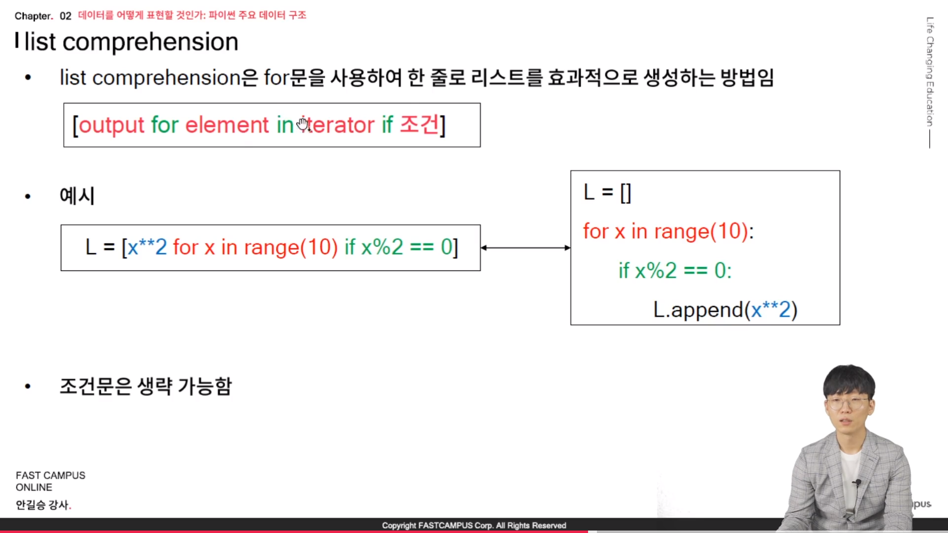
// 시트명 정의는 list comprehension 을 통해서 작업을 한다.
// skiprows 를 설정했다는 것은 6행까지 불러 오지 않는 것이다.
// concat 을 이용해서 데이터를 붙여 준다.
* Step 2. 포맷 통일 및 변수 추가
- 일자 컬럼이 YYYY-MM-DD 라는 포맷의 날짜와 YYYY.MM.DD 라는 포맷의 날짜가 혼합되어 있어, 원활한 분석을 위해 포맷을 통일해야 한다.
- 품명과 수량 컬럼을 바탕으로 주문 금액을 계산하여, 주문 금액이라는 컬럼을 추가
- 제품에 따른 가격 정보는 제품별_가격정보.xlsx 에 정의되어 있다.
// 위와 같은 데이터를 처리하기 위해서 새로운 문법이 필요하다.
* 새로운 문법 (1/2)
- Series.to_dict( ) : Series 의 index 를 Key 로, data 를 Valu로 하는 사전으로 변환
// 이렇게 바꿔주는 이유는 replace 를 사용해서 dictonary 를 사용하기 위한 것이다.
- Series.replace(dict) : Series에 있는 값 가운데 dict 의 key 의 값이 있으면 대응되는 value 로 변환
* 새로운 문법 (2/2)
- .T : 행과 열을 바꾼 전치 행렬을 반환한다는 것이다.
- DataFrame 에 새로운 컬럼 추가 : df['새로운 컬럼명'] = 연산 결과
* 실습
// . 을 - 으로 바꾸거나 - 을 . 로 바꾸거나 할 수 있다. str ( ) 을 사용하게 되면 str 에 들어있는 내장함수를 사용할 수 있다. series 의 replace 와 함수와 우연히 이름이 같을 뿐이다.
// 원활한 분석을 위해, 행과 열을 바꿀 필요가 있다. 하나의 행이나, 열에는 하나의 자료 구조가 들어가는 것이 좋다.
// T 를 이용해서 frame의 형태를 바꿔주는 것이다.
// 새로운 데이터 프레임의 컬럼명에 따라서 작업을 해야 하고, 또 to_dict( ) 를 사용해서 series를 dicationary 형태로 바꾸는 것이다.
// replace : 품명 컬럼에 price dict 의 key 가 있으면 value로 바꾼다.
// ndarray 브로드캐스팅 => 유니버셜 함수
* Step 3. 월별 매출 추이 파악
- 일자 변수를 바탕으로 월을 추출한 뒤, 월을 x축으로 주문 금액 및 품목별 주문 금액을 y 축으로 하는 꺽은선 그래프를 그린다.
* 실습
// 일자변수가 object type 이므로 split을 하더라도 object 여서 astype 으로 int 로 적용해준다.
// %matplotlib inline magic keyword !! 기억하자!!!
// unique( ) 을 써서 각각의 리스트 값을 나타내주고.. 축에서 나타낼 때는 통일
// 마스킹 검색을 이용할 수 있다.
* Step 4. 다양한 조건에 따른 판매 통계 분석
- 제품별 판매량 합계를 나타내는 막대 그래프와 제품과 결제 수단에 따른 히트 맵을 그린다.
* 실습
// 각각의 데이터를 처리하고 나서.. hist 를 그린다.
* Step 5. 충성 고객 찾기
- 주문 금액 합과 빈도가 각각 상위 10% 안에 속하는 고객을 찾아서 정리하는 것이다.
* 실습
// cond 1 = 을 만족하는 여부.. cond2 = 을 만족하는 여부로 결정하고 나서.
// loc [ cond1 & cond2 ] 등으로 찾을 수가 있다.
[파이썬을 활용한 데이터 전처리 Level UP-Comment] - 파이트차트, 박스 플롯 및 실제 프로젝트를 통해서 내용을 알아 볼 수 있었다.
- 마스킹 검색, 문자열 검색, matplotlib 에 대한 기초 이론 등에 대해서 배웠었다. 특히, matplotlib 은 기초 이론만 습득을 했어고 아마도 오늘 실습을 통해서 자세히 알아 나갈 것 같다.
[01. Part 1) 데이터 핸들링Chapter 06. 데이터 이쁘게 보기 - 데이터 시각화 - 02. 꺽은선 그래프 그리기]
// 산점도는 분포를 확인하기 용이한 그래프이다.
* matplotlib을 이용한 꺽은선 그래프 그리기
- pyplot.plot 함수를 사용하면 꺽은선 그래프를 그릴 수 있음 - 주요 입력 . x, y : x, y 축에 들어갈 값 (iterable 한 객체여야 하며, x[ i ] , y[ i ] 가 하나의 점이 되므로 길이가 같아야 한다.)
// series 등 점의 길이가 같아야 된다. . linewidth : 선 두께 . marker : 마커 종류 . markersize : 마커 크기 . color : 선 색상 . linestyle : 선 스타일 . label : 범례
* Pandas 객체의 method를 이용한 꺽은선 그래프 그리기
- DataFrame.plot( ) 함수를 사용하면 DataFrame 을 사용한 그래프를 그릴 수 있다. - 주요 입력 . kind : 그래프 종류 (‘line' 이면 선 그래프를 그림) . x : x 축에 들어갈 컬럼명 (입력하지 않으면, index 가 x 축에 들어간다.) . y : y 축에 들어갈 칼럼명 (목록) . xticks, yticks 등도 설정이 가능함 (단, pyplot을 사용해서도 설정이 가능하다.)
* 실습
// 기본 환경 설정
// numpy 도 같이 불어옴
// magic keyword %matplotblib inline 을 통해서 cell 에서 그래프 표시
// Malgun Gothic => 보통은 윈도우 환경이다.
// cumsum 누적합이다.
// plt.xticks(xtick_range, df['날짜'].loc[xtick_range] x 축을 정의한다.
// DataFrame으로 직접 그래프 그리기는.. df.plot(kind='line', x='날짜', y = ['상품1, '상품2', '상품3'] 으로 설정하여 그릴 수가 있다.
// DafatFrame의 경우에는 훨씬 더 편하지만, 환경 설정등은 기본 환경을 이용해서 설정해줘야 한다.
// groupby 으로 그래프 그리기
// groupby , pivot 은 그래프를 그리기 위해서 많이 쓰이고 있다.
* matplotlib 을 이용한 산점도 그리기
- pyplot.scatter 함수를 사용하면 산점도를 그릴 수 있다.
- 주요 입력
. x, y: x, y 축에 들어갈 값 (iterable한 객체여야 하며, x[ i ], y[ i ] 가 하나의 점이 되므로 두 입력의 길이가 같아야 한다.
. marker : 마커 종류
. markersize : 마커 크기
. color : 마커 색상
. label : 범례
// 솔직히 matplotlib 함수에 대서는 자료가 굉장히 많이 있다.
// 아래는 matplotlib documentation 을 검색했을 때 나오는 공식 사이트
The horizontal / vertical coordinates of the data points.xvalues are optional and default torange(len(y)).
Commonly, these parameters are 1D arrays.
They can also be scalars, or two-dimensional (in that case, the columns represent separate data sets).
These arguments cannot be passed as keywords.
fmtstr, optional
A format string, e.g. 'ro' for red circles. See theNotessection for a full description of the format strings.
Format strings are just an abbreviation for quickly setting basic line properties. All of these and more can also be controlled by keyword arguments.
This argument cannot be passed as keyword.
dataindexable object, optional
An object with labelled data. If given, provide the label names to plot inxandy.
Note
Technically there's a slight ambiguity in calls where the second label is a validfmt.plot('n','o',data=obj)could beplt(x,y)orplt(y,fmt). In such cases, the former interpretation is chosen, but a warning is issued. You may suppress the warning by adding an empty format stringplot('n','o','',data=obj).
// 이외에도 다양한 paramter 값 들이 있다.
Other Parameters:
scalex, scaleybool, default: True
These parameters determine if the view limits are adapted to the data limits. The values are passed on toautoscale_view.
// 상기와 같은 많은 기능들을 다 사용할 수는 없었지만, matplotlib 을 이용해서는 stock chart 를 나타내는 것에는 한계가 다분히 존재한다. 그래서 다른 candle stick 을 그릴 수 있는 plot 이 더 좋았고, 요즘에는 active chart 인 plotly 를 더욱 많이 사용하는 것 같다.
// candlestcik chart 그리기 좋은 라이브러리. pip install 을 통해서 설치 하면된다.
// 난 개인적으로 요즘 plotly 가 더 좋지만. ^^;;
[01. Part 1) 데이터 핸들링Chapter 06. 데이터 이쁘게 보기 - 데이터 시각화 - 03. 산점도 그리기]
* Pandas 객체의 method 를 이용한 산점도 그리기
- DataFrame.plot( ) 함수를 사용하면 DataFrame을 사용한 그래프를 손쉽게 그릴 수 있으며, 산점도 역시 그릴 수 있다.
- 주요 입력
. kind : 그래프 종류 ( 'scatter'면 산점도를 그린다.)
. x : x 축에 들어갈 컬럼명 (입력하지 않으면, index 가 x 축에 들어간다.)
. y: y 축에 들어갈 컬럼명
. xticks. yticks 등도 설정이 가능하다. (단, pyplot 을 사용해서도 설정이 가능하다)
* 실습
// 그래프를 그리는 것은 쉬운편이나, 그래프를 그리기 위해서 데이터를 어떤식으로 정제를 해야 하는지를 잘 알아야 한다.
// string access 를 통해서 하는가, 글씨 두개를 날리던가 하는 식으로 원하는 형태의 string을 얻을 수 있다.
// multiindex 는 . groupby 에서 list 형태 일때는 as_index 를 True로 두면된다. 약간 까다롭기 때문에 일반적으로 False로 두고 작업을 하는 것이 좋다.
// .unique( ) 를 통해서 각각의 리스트를 돌면서.. scatter 를 찍게 된다.
// Datafrme 을 이용해서 그리기
// .add_suffix 모든 것에 대해서 접미사를 붙이는 것이다.
// unique 한 갯수를 가지는 list 형태이다.
// df.plot 형태로 기본적인 plot의 형태를 찍어줬다.
// 산점도는 그래프를 그리는 것도 보다도 그래프를 그리기 위해서 데이터를 정리하는 시간이 더 오래 걸린다.
[01. Part 1) 데이터 핸들링Chapter 06. 데이터 이쁘게 보기 - 데이터 시각화 - 04. 막대 차트 그리기]
* matplotlib 을 이용한 막대 차트 그리기
- pyplot.bar 함수를 사용하면 막대 차트를 그릴 수 있다.
- 주요 입력
. x : 막대의 위치
. height : 막대의 높이
. width : 막대의 너비
// 추후에는 width를 넓히는 것이 더 중요하는 것을 의미한다.
. align : 막대 정렬
* Pandas 객체의 method 를 이용한 막대 차트 그리기
- DataFrame.plot( ) 함수를 사용하면 DataFrame을 사용한 그래프를 손쉽게 그릴 수 있으며, 막대 차트 역시 그릴 수 있다.
- 주요입력
. kind: 그래프 종류 ('bar'면 막대 그래프를 그린다.)
. x: x축에 들어갈 컬럼명 (입력하지 않으면, index가 x축에 들어감)
. y : y 축에 들어갈 컬럼명 (목록)
. xticks, yticks 등도 설정이 가능하다. (단, pyplot 을 사용해서도 설정이 가능하다.)
* 실습
// x 에 문자를 넣게 되면 위치는 자동으로 0, 1, 2, 3, ~~~ 이런식으로 자동으로 잡히게 된다.
* 다중 막대 그래프 그리기
- 다중 막대그래프는 pandas의 groupby 혹은 set_index, 그리고 unstack, 혹은 pivot_table을 사용하면 쉽게 그릴 수 있다.
// 오른쪽과 같은 그래프가 다중 막대 그래프를 그리기 좋은 구조이다.
// pivot table 을 이용해서 만들면 되고, 만약에 안된다고 하면 groupby 를 사용해서 작업을 하면 된다.
* 실습
// groupby 이후에 unstack 을 하게 되면 pivot 형태를 가지게 되고 이를 그래프로 나타내면 된다.
[파이썬을 활용한 데이터 전처리 Level UP-Comment] - matplotlib 을 이용한 그래프 그리그에 대해서 배워 볼 수 있었다. bar, line, scatter 등에서 배울 수 있었고 각각 DataFrame 을 사용해서 어떻게 작업을 해서 plot 을 그려야 할지에 대해서 알아봤다.
dtypedata type, or dict of column name -> data type
Use a numpy.dtype or Python type to cast entire pandas object to the same type. Alternatively, use {col: dtype, …}, where col is a column label and dtype is a numpy.dtype or Python type to cast one or more of the DataFrame’s columns to column-specific types.
copybool, default True
Return a copy whencopy=True(be very careful settingcopy=Falseas changes to values then may propagate to other pandas objects).
errors{‘raise’, ‘ignore’}, default ‘raise’
Control raising of exceptions on invalid data for provided dtype.
raise: allow exceptions to be raised
ignore: suppress exceptions. On error return original object.
[01. Part 1) 데이터 핸들링Chapter 06. 데이터 이쁘게 보기 - 데이터 시각화 - 01. matplotlib 기초]
// python 에서 대중적으로 쓰는 시각화 모듈이다.
* matplotlib 이란
- 파이썬에서 차트나 플롯으로 데이터를 시각화하기 위한 모듈로 사용이 간편하고 다양한 그래프를 제공해서 많이 사용된다.
// seaborn, boat ??? 그런 프로그램이 있다.
- matplotlib을 이용해서 그릴 수 있는 대표적인 그래프는 다음과 같다.
. 꺽은선 그래프 -> line plot
. 산점도 -> scatter plot
. 막대 그래프 -> bar chart
. 히스토그램 -> histogram
. 박스 플롯 -> box plot
- pandas 의 객체에서도 메서드로 matplotlib의 함수를 사용할 수 있다.
// pandas 에서도 사용할 수 있다. 그 의미는 굳이 matplotlib 을 import 하지 않고, pandas에서 불러와서 쓸수 있다는 것이다.
* 기초 환경 설정
- pyplot.rcParams 를 이용한 폰트 설정 및 그래프 크기 설정
// 기본적인 환경을 셋팅하는 함수라고 보면된다.
. rcParams['font.family'] : 폰트 설정 (특히, 한글을 쓰는 경우에 반드시 설정 필요)
// matplotlib 에서는 한글을 지원하지 않기 때문에 네모박스처럼 알아 볼 수 없는 것으로 나온다.
. rcParams['font.size'] : 글씨 크기 설정
. rcParams['figure.figsize'] : (x, y) 꼴의 튜플로 그래프의 크기를 설정
// 10, 5 정도로 하면 적당한 그림의 크기기 나온다고 보면 된다.
* 쥬피터에서 그래프 그리기
- 쥬피터의 매직 키워드인 %matplotlib inline을 이용하면 셀에 그래프를 직접 출력할 수 있다.
- 쥬피터를 사용하지 않는 경우에는 plt.figure( ) 를 사용해서 그래프 객체를 일일이 생성하고 저장해야 하지만, 쥬피터에서는 한 셀에서 그래패를 그릴 떄마다 하나의 객체가 생성된다.
// 이 강의에서는 jupyter notebook을 기초로 하기 때문에 failed show 등에 대해서는 다루지 않는다.
. 한 셀에서 plt의 함수를 사용하여 그래프를 그리면 하나의 객체에 누적해서 그래프가 생성된다.
// 중첩을 하지 않기 위해서는 각 셀을 나눠서 plt 를 작업을 해야 한다.
. 그래프를 다 그린 후에는 plt.savefig(file, dpi) 를 사용하여 그래프를 저장할 수 있다.
// dpi 는 보통 300 으로 설정한다.
* 자주 사용되는 색상 설정
- 다양한 그래프에서 색상을 설정해야 하며, 자주 사용되는 색상 및 입력은 다음과 같다.
// 직관적으로 결과를 보기 때문에 색상에는 크게 신경쓰지는 않는다.
* 자주 사용되는 마커 및 선 스타일 설정
- 마커란 하나의 데이터 포인트 (샘플)을 나타내는 기호를 나타낸다.
- 선 스타일은 꺽은선 그래프의 선 스타일을 의미한다.
// 별, 더하기, 다이아몬드 등을 주로 쓴다.
* label 및 title 설정
- label 이란 축의 이름을 의미하며, plt.xlabel과 plt.ylael을 사용하여 정의할 수 있다.
. plt.xlabel(label, **kwargs) : label (str) 로 xlabel을 설정
. plt.ylabel(label, **kwargs) : label (str) 로 ylabel을 설정
. **kwargs : 텍스트의 특성을 설정하는 키워드 (예: fontproperties, fontsize, fontstyle 등)
// 앞서봤던 기초 환경에서 쓰는 rcParams와 달리 keyword로 의한 텍스트 특성은 라벨을 적용할 때 쓰이는 것이다.
- title 이란 그래프의 이름으로, plt.title 을 사용하여 정의 할 수 있다.
. plt.title(label, loc) : label (str) 로 title 을 설정 (loc : 위치 {'center', 'left', 'right'})
// loc 은 잘 설정하지 않는다. 주로 center
* tick 설정
- tick이란 그래프에서 나타내는 눈금을 의미하며, plt.xticks와 plt.yticks을 이용하여 설정할 수 있다.
. plt.xticks(ticks, lables) : ticks (위치)에 labels를 입력 (x축)
. plt.yticks(ticks, lables) : ticks (위치)에 labels를 입력 (y축)
- 사용 예시 : plt.xticks([1,2,3,4,5], ['a', 'b', 'c', 'd', 'e'])
* legend 설정
- legend (범례)를 표시하려면 plt.legend(loc)을 사용하여 범례를 표시할 수 있다.
. loc : 범례 위치 {'upper right' (1), 'upper left' (2), ....}
- 단, 범례를 표시하려면 그래프를 그릴 때 label 키워드를 사용하여 범례를 정의해야 한다.
* 축 범위 설정
- plt.xlim(left, right) : x축의 범위를 (left, right) 로 설정
- plt.ylim(bottom, top) : y 축의 범위를 (bottom, top) 로 설정
[파이썬을 활용한 데이터 전처리 Level UP-Comment] 마스킹 검색과, 문자열 검색 기본적인 문법에 대해서 배워 볼 수 있었다. matplotlib 에 대해서는 기초적인 이론을 배웠고 추후 강의시간에 실습을 통해서 적용해 볼 수 있을 것이다.
Used to determine the groups for the groupby. Ifbyis a function, it’s called on each value of the object’s index. If a dict or Series is passed, the Series or dict VALUES will be used to determine the groups (the Series’ values are first aligned; see.align()method). If an ndarray is passed, the values are used as-is determine the groups. A label or list of labels may be passed to group by the columns inself. Notice that a tuple is interpreted as a (single) key.
axis{0 or ‘index’, 1 or ‘columns’}, default 0
Split along rows (0) or columns (1).
levelint, level name, or sequence of such, default None
If the axis is a MultiIndex (hierarchical), group by a particular level or levels.
as_indexbool, default True
For aggregated output, return object with group labels as the index. Only relevant for DataFrame input. as_index=False is effectively “SQL-style” grouped output.
sortbool, default True
Sort group keys. Get better performance by turning this off. Note this does not influence the order of observations within each group. Groupby preserves the order of rows within each group.
group_keysbool, default True
When calling apply, add group keys to index to identify pieces.
squeezebool, default False
Reduce the dimensionality of the return type if possible, otherwise return a consistent type.
Deprecated since version 1.1.0.
observedbool, default False
This only applies if any of the groupers are Categoricals. If True: only show observed values for categorical groupers. If False: show all values for categorical groupers.
New in version 0.23.0.
dropnabool, default True
If True, and if group keys contain NA values, NA values together with row/column will be dropped. If False, NA values will also be treated as the key in groups
New in version 1.1.0.
// groupby 의 parameter 또한 다양하게 존재한다. dropna 의 경우에도 자주 사용하는 것 중에 하나이다.
[01. Part 1) 데이터 핸들링 Chapter 05. 보고 싶은 데이터 찾아보기 - 데이터 정렬과 인덱싱 - 01. 데이터 정렬]
* 리스트 및 튜플 정렬
- sort: 리스트 및 튜플 자체를 정렬 (return 값이 없음)
. reverse : 내림차순으로 정렬할 것인지 여부를 결정하는 매개 변수
. Pandas 에서 inplace = True 로 설정한 것과 같다고 볼 수 있다.
- sorted: 정렬된 리스트 및 튜플을 반환
. reverse : 내림차순으로 정렬할 것인지 여부를 결정하는 매개 변수
. key : 정렬 기준 함수 (주로 lambda 함수를 사용)
// lambda 는 길이가 길지 않기 때문에 lambda 를 사용한다.
* 실습
// L.sort( ) 한다고 해서 출력이 안된다.
// L 을 별도로 찍어줘야 한다.
// lambda 를 이용해서 어떤 요소를 기준으로 정렬할 수가 있다.
// lambda 를 abs(절대값) 을 기준으로 정렬하는 것이다. 3에 가까울수록 앞쪽으로 정렬된다.
// reverse = True 을 줘서 길이를 기준으로 내림차순 정렬하는 것이다.
* Series 정렬
- sort_values 를 사용하면 Series를 손쉽게 정렬할 수 있다.
- 주요 입력
. ascending: 오름차순으로 정렬할 것인지 여부
// True: 오름 차순, False: 내림 차순
. key : 정렬 기준 함수 (주로 lambda 함수를 사용)
. na_position -> 결측이 있는 경우 어디에 배치할 것인지 결정 {first, last}
Choice of sorting algorithm. See also ndarray.np.sort for more information.mergesortis the only stable algorithm. For DataFrames, this option is only applied when sorting on a single column or label.
na_position{‘first’, ‘last’}, default ‘last’
Puts NaNs at the beginning iffirst;lastputs NaNs at the end.
ignore_indexbool, default False
If True, the resulting axis will be labeled 0, 1, …, n - 1.
New in version 1.0.0.
keycallable, optional
Apply the key function to the values before sorting. This is similar to thekeyargument in the builtinsorted()function, with the notable difference that thiskeyfunction should bevectorized. It should expect aSeriesand return a Series with the same shape as the input. It will be applied to each column inbyindependently.
New in version 1.1.0.
* DataFrame 중복 제거
- drop_duplicates 함수를 사용하면 중복이 있는 행을 제거할 수 있다.
- 주요 입력
. subset: 중복 기준을 판단하는 컬럼 (목록)
. keep: 중복이 있는 어느 부분을 남길 것인지 결정 {'first', 'last', 'false'}
.. first : 첫 번째 행을 남김
.. last : 마지막 행을 남김
.. false : 중복 행을 모두 제거
* 실습
// A를 기준으로 중복된 값 제거 A를 기준으로 unique 한 값에 따라서 남는다. Default 가 first 이므로 첫행이 살아 있는 것이다.
// pandas.DataFrame.drop_duplicates 의 documentation
subsetcolumn label or sequence of labels, optional
Only consider certain columns for identifying duplicates, by default use all of the columns.
keep{‘first’, ‘last’, False}, default ‘first’
Determines which duplicates (if any) to keep. -first: Drop duplicates except for the first occurrence. -last: Drop duplicates except for the last occurrence. - False : Drop all duplicates.
inplacebool, default False
Whether to drop duplicates in place or to return a copy.
ignore_indexbool, default False
If True, the resulting axis will be labeled 0, 1, …, n - 1.
[01. Part 1) 데이터 핸들링 Chapter 05. 보고 싶은 데이터 찾아보기 - 데이터 정렬과 인덱싱 - 02. 인덱서를 활용한 인덱싱]
// 데이터 시리즈를 할때 한번 했었지만 다시 리마인드 한다는 생각으로, 하지만, 중요한 내용이기때문에. 다시 한번 상기
* 인덱싱과 슬라이싱 (remind)
- 판다스의 객체는 암묵적인 인덱스(위치 인덱스)와 명시적인 인덱스라는 두 종류의 인덱스가 있어, 명시적인 인덱스를 참조하는 loc 인덱서와 암묵적인 인덱스를 참조하는 iloc 인덱서가 존재한다.
// 암묵적..인덱스는 사용자가 설정한 것이 아니고, 명시적 인덱스는 사용자가 직접 설정한 것이라고 이해하면 된다.
// 데이터프레임일때는 리스트나 컬럼으로 접근
* 값 변경하기 (remind)
- 인덱서를 사용하여 조회한 값을 직접 변경할 수 있다.
// 판다스에 있는 자료를 바꿀 때는 반드시 인덱서를 사용해야 한다.
// 이 외에도 방법은 있지만, 반드시 사용해야 한다고 기억해야 한다.
// loc[c, col2] 으로도 동일한 기대값을 가질 수 있다.
* 인덱서를 사용해야 하는 이유
- DataFrame의 값을 바꾸는 경우에는 가장 자주 흔히 보는 경고로 SettingWithCopyWarning이 있다.
// warning 은 많이 보아왔다.
- df['A'] 는 view를 반환하고, df.loc['A'] 는 copy된 값을 반환한다.
// loc[a] 에 저장하면 df 자체가 바뀔 수 없고, 값을 바꾸게 되면 df 자체가 바뀐다.
. view 를 반환한 결과를 바꾸는 경우에는 원본 자체도 변경이 일어날 수 있다.
. copy를 반환한 결과를 바꾸더라도 원본에는 변경이 없다.
- 따라서 view를 반환하지 않도록 가능하면 인덱서를 사용해야만, 사용자의 의도대로 DataFrame을 변경할 수 있다.
[파이썬을 활용한 데이터 전처리 Level UP-Comment] groupb_by 함수의 경우에는 데이터 처리에 있어서 굉장히 많이 사용하는 것을 보아왔다. 어떤식으로 묶어서 보는냐에 따라서 다양한 insight 가 나오게 된다. 그래서 더욱더 어렵다. 그 모든것의 판단은..역시 경험? 하.. 어렵구만...
objs a sequence or mapping of Series or DataFrame objects
If a mapping is passed, the sorted keys will be used as thekeysargument, unless it is passed, in which case the values will be selected (see below). Any None objects will be dropped silently unless they are all None in which case a ValueError will be raised.
axis {0/’index’, 1/’columns’}, default 0
The axis to concatenate along.
// axis 는 default가 0 이다. 굳이 작성하지 않으면 row 형태로 밑으로 붙는 것이다.
[Chapter 04. 한 눈에 데이터 보기 - 데이터 통합 및 집계 - 03. 기초 통계 함수를 활용한 데이터 집계]
* 다양한 기초 통계 함수
- 기초 통계 함수는 DataFrame와 Series에 대해 모두 정의되어 있다.
. sum -> 합계 계산
. mean -> 평균 계산
. std -> 표준편차 계산
// std, standard devation
. var -> 분산 계산
. quantile -> 사분위수 계산
. min -> 최소값 계산
. max -> 최대값 계산
// dataframe, series 의 method 로 활용 할 수 있다.
* Tip. Axis 키워드
- axis 키워드는 numpy 및 pandas의 많은 함수에 사용되는 키워드로, 연산 등을 수행할 때 축의 방향을 결정하는 역할을 한다.
- axis 가 0 이면 row 을, 1 이면 column 을 나타내지만 이렇게만 기억하면 논리적으로 이상한 점이 존재한다.
// 대부분의 열 기준 합이라는 것은 row 끼리, column 끼리
// concat 함수가 대표적인 함수이다.
* describe 함수
- 열별로 대표적인 기초 통계를 반환 (count, mean, std, min 25%, 50%, 75%, max)
// count 는 결측치를 제외한 결과를 보여준다.
// quantile(0.1) 상위 10% 값을 나타내는 것이다. 상위 10%라는 것은 작은 값 기준 10%라는 것이다.
// 데이터분석을 할때 어느정도로 분포가 되어있는지를 확인할 때 describe( ) 를 사용한다.
Descriptive statistics include those that summarize the central tendency, dispersion and shape of a dataset’s distribution, excludingNaNvalues.
Analyzes both numeric and object series, as well asDataFramecolumn sets of mixed data types. The output will vary depending on what is provided. Refer to the notes below for more detail.
// 결측치는 제외하고 값들을 보여 준다...
Parameters
percentileslist-like of numbers, optional
The percentiles to include in the output. All should fall between 0 and 1. The default is[.25,.5,.75], which returns the 25th, 50th, and 75th percentiles.
// 몇 번째에 해당하는지에 대한 사분위를 보여주는 것이다.
include‘all’, list-like of dtypes or None (default), optional
A white list of data types to include in the result. Ignored forSeries. Here are the options:
‘all’ : All columns of the input will be included in the output.
A list-like of dtypes : Limits the results to the provided data types. To limit the result to numeric types submitnumpy.number. To limit it instead to object columns submit thenumpy.objectdata type. Strings can also be used in the style ofselect_dtypes(e.g.df.describe(include=['O'])). To select pandas categorical columns, use'category'
None (default) : The result will include all numeric columns.
excludelist-like of dtypes or None (default), optional,
A black list of data types to omit from the result. Ignored forSeries. Here are the options:
A list-like of dtypes : Excludes the provided data types from the result. To exclude numeric types submitnumpy.number. To exclude object columns submit the data typenumpy.object. Strings can also be used in the style ofselect_dtypes(e.g.df.describe(include=['O'])). To exclude pandas categorical columns, use'category'
None (default) : The result will exclude nothing.
datetime_is_numericbool, default False
Whether to treat datetime dtypes as numeric. This affects statistics calculated for the column. For DataFrame input, this also controls whether datetime columns are included by default.
New in version 1.1.0.
[Chapter 04. 한 눈에 데이터 보기 - 데이터 통합 및 집계 - 04. pivot 을 이용한 데이터 집계]
* 피벗 테이블
- pivot table 은 데이터를 조건에 따른 변수들의 통계량을 요약한 테이블이다.
// 큰 데이터를 한 테이블로 나타낸다.
* pandas.pivot_table
- 주요 입력
. data -> 데이터 프레임
. index -> 행에 들어갈 조건
. columns -> 열에 들어갈 조건
. values -> 집계 대상 컬럼 목록
. aggfunc -> 집계 함수
* 실습
// index 제품, cloumns = , vlaues = , afffunc = 으로 ..하면 제품에 따른 것을 구하는 것이다.
If io is not a buffer or path, this must be set to identify io. Supported engines: “xlrd”, “openpyxl”, “odf”, “pyxlsb”, default “xlrd”. Engine compatibility : - “xlrd” supports most old/new Excel file formats. - “openpyxl” supports newer Excel file formats. - “odf” supports OpenDocument file formats (.odf, .ods, .odt). - “pyxlsb” supports Binary Excel files.
// engine 의 경우에는 openpyxl 을 자주 사용했었는데.. 정확히 어떠한 것이 더 유리한지를 모르겠다. memory 등 time loose 가 너무 심한건 아닌지.. 중복 코드도 의심해봐야 한다.
date_parserfunction, optional
Function to use for converting a sequence of string columns to an array of datetime instances. The default usesdateutil.parser.parserto do the conversion. Pandas will try to calldate_parserin three different ways, advancing to the next if an exception occurs: 1) Pass one or more arrays (as defined byparse_dates) as arguments; 2) concatenate (row-wise) the string values from the columns defined byparse_datesinto a single array and pass that; and 3) calldate_parseronce for each row using one or more strings (corresponding to the columns defined byparse_dates) as arguments.
// date_parser 도 은근히 많이 사용하는 option 중에 하나 인것 같은데..
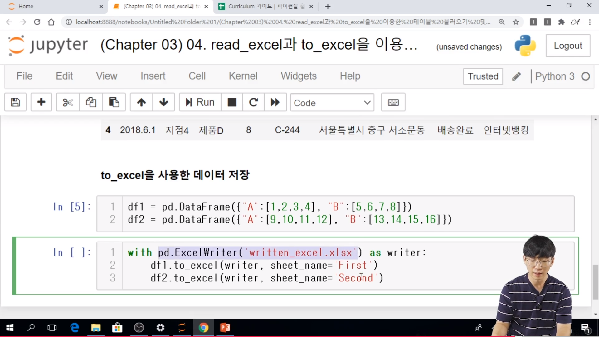
* to_excel 함수
- pandas의 to_excel 함수는 테이블 형태의 데이터를 저장하는데 효과적인 함수이다.
[Chapter 04. 한 눈에 데이터 보기 - 데이터 통합 및 집계 - 01. merge를 이용한 데이터 통합]
* merge가 필요한 상황
- 효율적인 데이터 베이스 관리를 위해서, 잘 정제된 데이터일지라도 데이터가 key 변수를 기준으로 나뉘어 저장되는 경우가 매우 흔하다.
// 공유하고 있는 key를 바탕으로 merge를 사용할 수가 있다.
* pandas.merge
// SQL로 치면 JOIN을 이용하는 것과 동일하다.
- key 변수를 기준으로 두 개의 데이터 프레임을 병함(join) 하는 함수이다.
- 주요 입력
. left -> 통합 대상 데이터 프레임1
. right -> 통합 대상 데이터 프레임2
. on -> 통합 기준 key 변수 및 변수 리스트 (입력을 하지 않으면, 이름이 같은 변수를 key 로 식별함)
// on 을 반드시 써주는 것이 좋다.
. left_on -> 데이터 프레임 1의 key 변수 및 변수 리스트
. right_on -> 데이터 프레임2의 key 변수 및 벼수 리스트
. left_index -> 데이터 프레임1의 인덱스를 key 변수로 사용할 지 여부
. right_index -> 데이터 프레임2의 인덱스를 key 변수로 사용할 지 여부
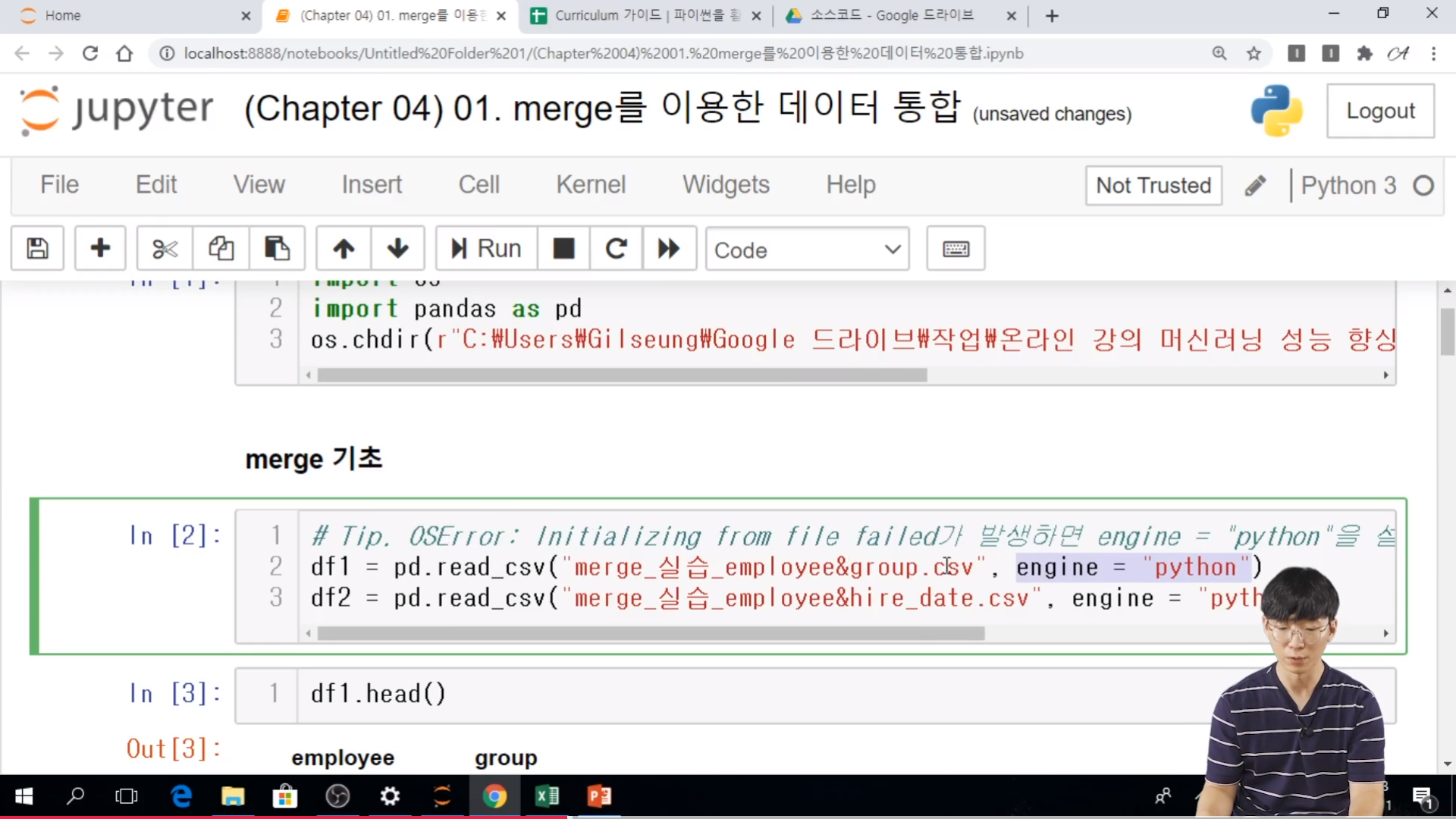
* 실습
- Tip.. engine = 'python' 은 OSError 를 피하기 위해서 사용하는 것인데. 느려진다는 단점이 있다. 하지만 그걸 예방하기 위해서 사용한다.
- 칼럼명이 같아서 key를 employee 로 인식함.
- on 을 사용해서 각각의 데이터 프레임을 사용할 수도 있고, list 형태로도 만들 수 있다.
- employee 와 name 이 colmun name 만 다르고 내용은 동일하다. 그래서 left_on, right_on 을 사용해서, merge를 할 수가 있다. 하지만, 이런 경우에는 각각의 key column 이 살아 있기 때문에... 지워져야 한다.
- dataframe 에서 컬럼은 axis =1 을 지정해줘야 한다.
- 불러 올때 index_col = 으로 설정해서 인덱스로 불러 올 수 있다.
- 이렇게 되면 right_index = True 값으로 정해줘야지 동일한 key 를 가지는 merge를 사용할수가 있다. 이런 경우에는 위에서 처럼 index 를 사용하지 않을 때 각각 생겨났던 column 이 생겨 나지 않는다. 이건 당연한 것이다. 왜냐하면 index 는 어떤 column 이 아니기 때문이다.
Changed in version 0.23.0:If data is a dict, argument order is maintained for Python 3.6 and later.
indexarray-like or Index (1d)
Values must be hashable and have the same length asdata. Non-unique index values are allowed. Will default to RangeIndex (0, 1, 2, …, n) if not provided. If both a dict and index sequence are used, the index will override the keys found in the dict.
dtypestr, numpy.dtype, or ExtensionDtype, optional
Data type for the output Series. If not specified, this will be inferred fromdata. See theuser guidefor more usages.
namestr, optional
The name to give to the Series.
copybool, default False
Copy input data.
=> 링크에 들어가서 살펴보면 상당히 많은 Attributes 들이 있는 것을 볼수 있다. 그중에서 자수 사용하는 것들은 몇 가지 정도가 아닐까 본다. 나도 아직 초보지만..ㅠ.ㅠ
Data structure also contains labeled axes (rows and columns). Arithmetic operations align on both row and column labels. Can be thought of as a dict-like container for Series objects. The primary pandas data structure.
Parameters
datandarray (structured or homogeneous), Iterable, dict, or DataFrame
Dict can contain Series, arrays, constants, or list-like objects.
Changed in version 0.23.0:If data is a dict, column order follows insertion-order for Python 3.6 and later.
Changed in version 0.25.0:If data is a list of dicts, column order follows insertion-order for Python 3.6 and later.
indexIndex or array-like
Index to use for resulting frame. Will default to RangeIndex if no indexing information part of input data and no index provided.
columnsIndex or array-like
Column labels to use for resulting frame. Will default to RangeIndex (0, 1, 2, …, n) if no column labels are provided.
dtypedtype, default None
Data type to force. Only a single dtype is allowed. If None, infer.
copybool, default False
Copy data from inputs. Only affects DataFrame / 2d ndarray input.
// 솔직히 pandas에서 dataframe을 빼면 속빈 강정아닌가? 어마무시하게 많이 쓰이는 데이터분석에서는 빠질수가 없다.
// attributes 및 method는 너무 많다... 패스
* 인덱싱과 슬라이싱
- 판다스의 객체는 암묵적인 인덱스(위치 인덱스)와 명시적인 인덱스라는 두 종류의 인덱스가 있어, 명시적인 인덱스를 참조하는 loc 인덱서와 암묵적인 인덱스를 참조하는 iloc 인덱서가 존재한다는 것이다.
- 암묵적인 인덱스는 자동으로 입혀진 인덱스라는 것이다.
- loc를 이용해서 슬라이싱에서는 맨 뒤 값을 포함한다.. 하지만, iloc의 경우에는 슬라이싱에서는 맨 뒤 값을 포함하지 않는 다는 것이다.
- 데이터 프레임의 컬럼 선택은 array 를 선택하는 것과 같다는 의미이다.
df[col_name] or df[col_name_list]
- 위치를 알고 싶을 때는 iloc indexer를 많이 쓴다.
* 실습
- loc => 사전에서 key를 가지고 value를 찾는 것과 완벽히 동일하다고 보면된다.
- loc 슬라이싱은 앞위 모두 포함..명시적인 값
- iloc 는 index number를 입력해준다. 맨뒤는 제외
- column name으로만 접근하면 => series로만 알려준다. df['a']
- column name list 로 접그하면 => dataFrame으로 알려준다. df[['a']]
* pandas의 값을 조회하기 (1/2)
- 쥬피터 환경에서는 데이터 프레임 혹은 시리즈 자료를 갖는 변수를 출력할 수 있다.
- Tip 1. pd.set_option('display.max_rows', None)을 사용하여, 모든 행을 보이게 할수 이 있음.
(None 자리에 숫자가 들어가면, 출력되는 행의 개수가 설정된다.)
- Tip 2. pd.set_option('display.max_columns', None) -> 모든 컬럼을 보이게 할 수 있음.
Python provides a.get()method to access adictionaryvalue if it exists. This method takes thekeyas the first argument and an optional default value as the second argument, and it returns the value for the specifiedkeyifkeyis in the dictionary. If the second argument is not specified andkeyis not found thenNoneis returned.
# without default
{"name": "Victor"}.get("name")
# returns "Victor"

{"name": "Victor"}.get("nickname")
# returns None

# with default
{"name": "Victor"}.get("nickname", "nickname is not a key")
# returns "nickname is not a key"
// get 메소드를 가끔은 사용할수도 있을 것 같다. 굳이 조건문을 통하지 않더라도 어떠한 dictionary 에 적당한 값이 있는지 없는지를 알기에도 적당할 듯한다.
// 전에 배운 list 형태에서 사용한 pop method 도 사용할 수 있다.
Python dictionaries can remove key-value pairs with the.pop()method. The method takes a key as an argument and removes it from the dictionary. At the same time, it also returns the value that it removes from the dictionary.
r-length tuples, in sorted order, with repeated elements
ExamplesResults
product('ABCD',repeat=2)
AAABACADBABBBCBDCACBCCCDDADBDCDD
permutations('ABCD',2)
ABACADBABCBDCACBCDDADBDC
combinations('ABCD',2)
ABACADBCBDCD
combinations_with_replacement('ABCD', 2)
AAABACADBBBCBDCCCDDD
- itertools.combinations(p, r)
. 이터레이터 객체 p에서 크기 r의 가능한 모든 조합을 갖는 이터레이터를 생성
Returnrlength subsequences of elements from the inputiterable.
The combination tuples are emitted in lexicographic ordering according to the order of the inputiterable. So, if the inputiterableis sorted, the combination tuples will be produced in sorted order.
Elements are treated as unique based on their position, not on their value. So if the input elements are unique, there will be no repeat values in each combination.
Roughly equivalent to:
def combinations(iterable, r):
    # combinations('ABCD', 2) --> AB AC AD BC BD CD
    # combinations(range(4), 3) --> 012 013 023 123
    pool = tuple(iterable)
    n = len(pool)
    if r > n:
        return
    indices = list(range(r))
    yield tuple(pool[i] for i in indices)
    while True:
        for i in reversed(range(r)):
            if indices[i] != i + n - r:
                break
        else:
            return
        indices[i] += 1
        for j in range(i+1, r):
            indices[j] = indices[j-1] + 1
        yield tuple(pool[i] for i in indices)
// 각 요소들을 조합해서 경우의 수에 대해서 모두 보여 주는 것이다. 이것 또한 잘 만 이용하면 좋을 것 같은데...
The code forcombinations()can be also expressed as a subsequence ofpermutations()after filtering entries where the elements are not in sorted order (according to their position in the input pool):
def combinations(iterable, r):
    pool = tuple(iterable)
    n = len(pool)
    for indices in permutations(range(n), r):
        if sorted(indices) == list(indices):
            yield tuple(pool[i] for i in indices)
The number of items returned isn!/r!/(n-r)!when0<=r<=nor zero whenr>n.
- itertools.permutations(p, r)
. 이터레이터 객체 p에서 크기 r의 가능한 모든 순열을 갖는 이터레이터를 생성
The code forpermutations()can be also expressed as a subsequence ofproduct(), filtered to exclude entries with repeated elements (those from the same position in the input pool):
def permutations(iterable, r=None):
    pool = tuple(iterable)
    n = len(pool)
    r = n if r is None else r
    for indices in product(range(n), repeat=r):
        if len(set(indices)) == r:
            yield tuple(pool[i] for i in indices)
// permutations function 안에서도 for 문과, if 문을 이용해서 tuple 형태로 반환해주고 있다.
* list comprehension
- list comprehension은 for문을 사용하여 한 줄로 리스트를 효과적으로 생성하는 방법임
- 예시
- 조건문은 생략 가능함.
* dictionary comprehension
- dictionary comprehension은 for문을 사용하여 한 줄로 사전을 효과적으로 생성하는 방법임
Chapter 02. 데이터를 어떻게 표현할 것인가 - 파이썬 주요 데이터 구조 - 02. Numpy의 데이터 구조
* 개요
- Numpy의 자료형은 ndarray로 효율적인 배열 연산을 하기 위해 개발되었음
- 리스트와 ndarray는 유연성과 효율성을 기준으로 비교할 수 있음
- list는 float, str 등 모든 요소를 저장할 수 있음
- ndarray 는 float, str 등을 정의해줘야 한다.
- ndarray 는 C로 구현된 내부 반복문을 사용하여 속도가 매우 빠른 편이다.
* 배열 만들기: np.array 함수
- np.array 함수를 사용하여 ndarray를 생성할 수 있음
// 사용하기 전에는 numpy 를 import 해줘야 한다.
import numpy as np
- np 로 as하는 것은 가장 많이 쓰는 약속 같은 것이다.
// numpy 에 대해서 cheat sheet 를 보는 것이 좋을 것 같아서 검색해보면 죄다. 어디로 연결되거나 길다....
- 2차원 배열인 경ㅇ, X[i, j]는 i행 j열에 있는 요소를 나타냄. (c.f. X가 리스트라면, X[i][j]로 접근함.)
- 부울 리스트도 인덱스로 사용할 수 있으며, True인 요소와 대응되는 요소만 가져옴
- 여러 개의 인덱스를 리스트 형태로 입력 받을 수도 있음
* 유니버셜 함수
- 유니버셜 함수는 ndarray의 개별 요소에 반복된 연산을 빠르게 수행하는 것을 주 목적으로 하는 함수
- ndarray x와 y에 대해, 덧셈, 뺄셈, 곱셈, 제곱 등 다양한 배열 간 이항 연산을 지원함.
- 유니버셜 함수는 단순 반복문에 비해, 매우 빠름
* 브로드캐스팅
- 다른 크기의 배열에 유니버셜 함수를 적용하는 규칙 집합으로, 큰 차원의 배열에 맞게 작은 배열이 확장됨.
- 첫번째 케이스와 두번째 케이스가 가장 많이 쓰인다.
- 첫번째 케이스에서 복제를 해서 각각 더한다.
- 브로드캐스팅 예시: z-normalization
* 비교 연산자
- 비교 연산자의 결과는 항상 부울 타입의 배열임
- 따라서 비교 연산자의 결과를 바탕으로 조건에 맞는 요소 탐색에 활용할 수 있음
sum(cond) - True는 1이고, False 0이기 때문에 더해도 개수가 나오게 된다.
[파이썬을 활용한 데이터 전처리 Level UP-Comment] 오늘 강의에서는 새로운 itertools 라는 구문에 대해서 배울 수 있었다. combination 기능을 잘만 이용하면 좀 더 빠른 연산을 할 수 있을 것 같기도 한데.. 불필요한 for 문이나 if 문 등 반복문과 조건문을 줄이기 위해서는 comprehension 문을 잘 사용하여야 하지만, 아직까지 그렇게 손에 있지 않는다. for 문 내에서도 다양한 조건 등을 걸어서 coding을 하다 보니 코딩만 더러워지고 있다. 거기에 time loose만 들어나고..
[Chapter 01. 시작에 앞서 데이터 전처리는 왜 중요할까 - 01. 데이터 전처리의 중요성 및 개요]
- 현실데이터는 분석 목적에 맞게 정리되어 있지않아, 데이터 분석 기법을 그대로 적용하기 어려움
* 현실 데이터 사례
- P 밸브사 - 수요 예측의 주문서 데이터가 파일명, 폴더 등이 정리되어 있지 않음.
- 포맷이 다른 주문서: 통일되지 않은 셀 위치와 제목 셀 이름이 정확하지 않음.
- 이런 경우에는 효과적으로 정리하는 방법이 필요함
- M공업사 - 설비 비가동 시점 예측
- 시간으로 정리되어 있으나 시간순서가 비정상적인 시간순서로 정리되어 있음- 기록되지 않은 알람이 포함되어 있음- 결측치 등이 다수 존재- 특수한 형태의 16진수로 구성된 리스트가 있음
- K홈쇼핑 - 매출 예측을 통한 방송 편성 최적화- 기존 홈쇼핑 방송 기록을 바탕으로 상품별 매출을 예측하고, 매출을 최대화하는 방향으로 방송을 편성하는 프로젝트- 불필요한 값이 너무 많아 데이터가 매우크고, 프로젝트 목표에 부합하지 않는 구조의 데이터임- 이와 같은 경우에는 잘 정리된것 처럼 보이지만 초심자의 경우에는 더 어려움을 느낄 수 있음
- 데이터 분석에 소요되는 시간- 모든 데이터 분석 프로젝트에서 데이터 전처리는 필수적인 과정이며, 많은 분석가들이 데이터 전처리에 가장 많은 시간을 투입함
. Cleaning and organizing data: 60%
. Collecting data sets: 19%
=> 이러한 결과를 바탕으로 전체 분석 시간의 79%를 사용한다고 한다. 전처리 역량이 분석 시간을 줄이는데 가장 중요하다는 의미이다.
// 하기사 코드를 짤때도 디버그야말로...진정한..시간잡아먹기.ㅠ.ㅠ
- 데이터 전처리의 주요 효과- 효율적인 분석을 가능하게 해준다.- 불필요한 정보를 제거함으로써 인사이트를 얻는데 도움이 된다.- 머신러닝 모델의 성능을 향상시킨다.
[Chapter 01. 시작에 앞서 데이터 전처리는 왜 중요할까 - 02. 데이터 전처리를 잘하는 방법]
* 경험을 쌓아라
- 데이터 전처리 역량을 쌓는 가장 확실한 방법은 좋은 경험을 많이 쌓는 것이다.
- 대다수의 경험은 "이런 방법을 쓰니까 시간만 날리더라. 다른 방법이 제일 좋았다"라는 레퍼런스가 됨
- 크롤링한 뉴스에서 단어 추철 및 변환하기 사례.. 데이터 추출하는 과제였는데.. 각각의 중요단어를 추출했어야 하지만.. 간단하게 띄워쓰기 등을 기준으로 했었다.
=> 형태소 분석 등등을 이용했어야 했다.
=> 실수를 통해서 지속적인 경험을 쌓아야지만 효과적인 방법으로 전처리를 할 수가 있다.
* 결과를 생각하라.
- 전처리의 결과인 전처리된 데이터의 구조를 미리 생각해야 불필요한 피드백 루프를 막을 수 있음
- 피드백 루프.. 처리된 데이터가 다시 돌아간다는 의미
* 처리 과정을 생각하라.
- 원 데이터를 결과 데이터로 바꾸기 위한 과정을 단계별로 정의해야 함
- 결과에 대해서 계획을 세워야 한다.
* 검색능력을 쌓아라.
- 데이터 전처리에 대한 기초적인 역량을 십분 발휘하기 위해서는, 필요한 전처리를 수행하는 방법을 검색하는 역량을 쌓아야 한다... 구글링을 많이 해라.
// 개인적으로도 네이버나 국내 검색엔진보다는 구글을 사용하는 것이 좋았다. 되도록이면 한글보다는 영어를 사용해서 전처리를 하는 것이 더 좋다.
- 검색쿼리 Tip: pytho, 모듈, how, 내용을 포함.
[Chapter 02. 데이터를 어떻게 표현할 것인가 - 파이썬 주요 데이터 구조 - 01. 리스트와 튜플]
패치#노트코딩, 주식, 자동매매, 백테스팅, 데이터분석 등 관심 블로그
비전공자이지만 금융 및 관련 프로그래밍에 관심을 두고 열심히 공부중입니다.
우리 모두 경제적 자유를 위해 성공해봅시다!!
※ 혹시, 블로그 내용중 문제되는 내용있으시면 알려주시면 삭제/수정 토록하겠습니다.
※ 모든 내용들은 투자 권유가 아니오니 참고만 하시고, 또한 출처는 모두 표기토록 노력하겠으나 혹시 문제가 되는 글이 있다면 댓글로 남겨주세요~^^