[패스트캠퍼스 수강 후기] 데이터전처리 100% 환급 챌린지 27회차 미션 Programming/Python2020. 11. 28. 12:52
[파이썬을 활용한 데이터 전처리 Level UP- 27 회차 미션 시작]
* 복습
- sklearn.impute.SimpleImputer, fillna를 이용해서 ffill, bfill 처리
- 결측치 예측 모델 활용 방법
[04. Part 4) Ch 18. 문자보다는 숫자 범주형 변수 문제 - 01. 문제 정의 및 해결 방법]

* 문제 정의
- 데이터에 범주형 변수가 포함되어 있어, 대다수의 지도 학습 모델이 학습되지 않거나 비정상적으로 학습되는 문제를 의미
. str 타입의 범주형 변수가 포함되면 대다수의 지도 학습 모델 자체가 학습이 되지 않음
. int 혹은 float 타입의 범주형 변수는 모델 학습은 되나, 비정상적으로 학습이 되지만, 입문자는 이를 놓치는 경우가 종종있다.
- 모델 학습을 위해 범주형 변수는 반드시 숫자로 변환되어야 하지만, 임의로 설정하는 것은 매우 부적절하다.
. (예시) 종교 변수 : 기독교 = 1, 불교 = 2, 천주교 =3
불교는 기독교의 2배라는 등의 대수 관계가 실제로 존재하지 않지만, 이처럼 변환하면 비상적인 관계가 생성된다.
// 적절한 숫자로 변화 되어야 한다.
- 특히, 코드화된 범주형 변수도 적절한 숫자로 변환해줘야 한다.
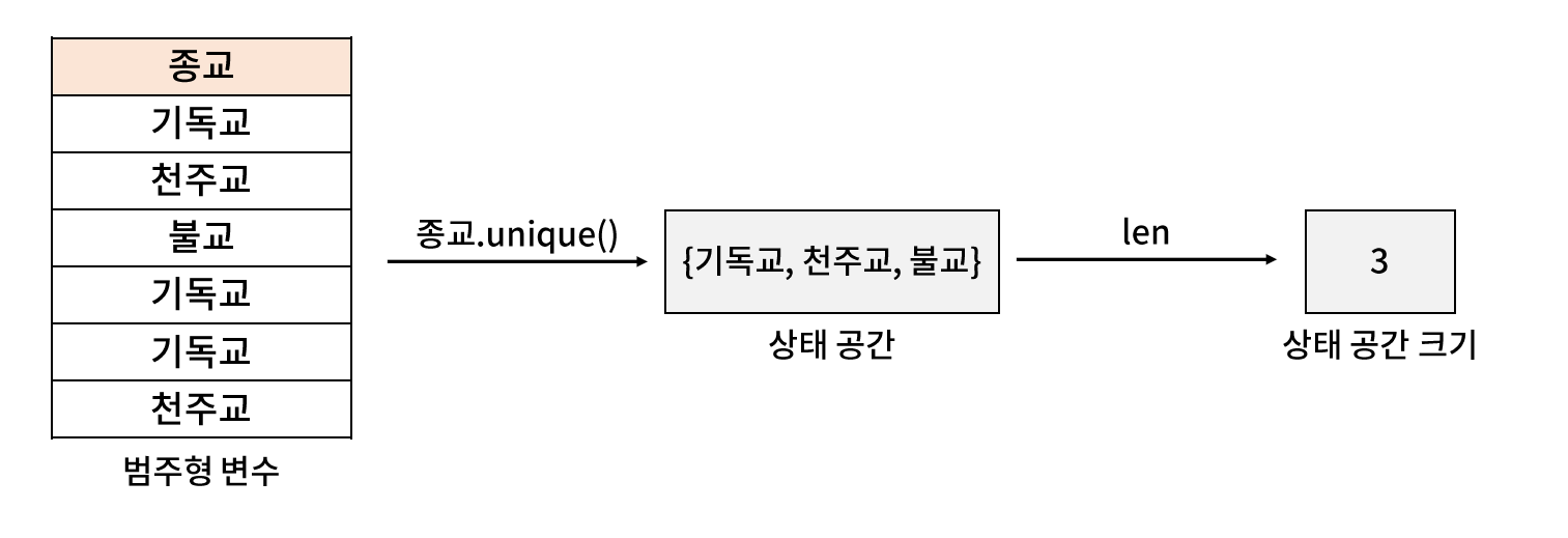
* 범주형 변수 판별
- 범주형 변수는 상태 공간의 크기가 유한한 변수를 의미하며, 반드시 모데인이나 변수의 상태 공간을 바탕으로 판단해야 한다.
- int 혹은 float 타입으로 정의된 변수는 반드시 연속형 변수가 아닐 수 있다는 점에 주의해야 한다.
- (예시) 월(month)은 비록 숫자지만 범주형 변수이다.
* 범주형 변수 변환 방법 (1) 더미화
- 가장 일반적인 범주형 변수를 변환하는 방법으로, 범주형 변수가 특정 값을 취하는지 여부를 나타내는 더미 변수를 생성하는 방법

// 추론할 수 있기 때문에.. 있으나마나한 데이터이기 때문에 그렇다.
// Tree 계열에서는 설명력을 위해서 넣는 경우도 있다.
* 범주형 변수 변환 방법 (2) 연속형 변수로 치환
- 범주형 변수의 상태 공간 크기가 클 때, 더미화는 과하게 많은 변수를 추가해서 차원 저주 문제로 이어질 수 있다.
- 라벨 정보를 활용하여 범주 변수를 연속형 변수로 치환하면 기존 변수가 가지는 일부 손실될 수 있고 활용이 어렵다는 단점이 있으나, 차원의 크기가 변하지 않으며 더 효율적인 변수로 변환할 수 있다는 장점이 있다.

[04. Part 4) Ch 18. 문자보다는 숫자 범주형 변수 문제 - 02. 관련 문법 및 실습]

* Series.unique( )
- Seires 에 포함된 유니크한 값을 반환해주는 함수로, 상태 공간을 확인하는데 사용
* feature_engine.categorical_encoders.OneHotCategoricalEncoder
- 더미화를 하기 위한 함수로, 활용 방법은 sklearn 의 인스턴스의 활용 방법과 유사하다.
- 주요 입력
. variables : 더미화 대상이 되는 범주형 변수의 이름 목록 (주의 : 해당 변수는 반드시 str 타입이어야 한다.)
. drop_last : 한 범주 변수로부터 만든 더미 변수 가운데 마지막 더미 변수를 제거할 지를 결정
. top_categories : 한 범주 변수로부터 만드는 더미 변수 개수를 설정하며, 빈도 기준으로 자른다.
- 참고 : pandas.get_dummies( ) 는 이 함수보다 사용이 휠씬 간단하지만, 학습 데이터에 포함된 범주형 변수를 처리한 방식으로 새로 들어온 데이터에 적용이 불가능하기 때문에, 실제적으로 활용이 어렵다.
* 실습

// 범주형 변수 들을 판별 하고 난 다음에 더미화를 이용해서 범주 변수들을 처리 한다.
// pandas.Series.unique Documentation
pandas.pydata.org/pandas-docs/stable/reference/api/pandas.Series.unique.html
Series.unique()Return unique values of Series object.
Uniques are returned in order of appearance. Hash table-based unique, therefore does NOT sort.
Returns
ndarray or ExtensionArray
The unique values returned as a NumPy array. See Notes.
// feature_engine.categorical_encoders.OneHotCategoricalEncoder Documentation
feature-engine.readthedocs.io/en/latest/encoders/OneHotCategoricalEncoder.html
classfeature_engine.categorical_encoders.OneHotCategoricalEncoder(top_categories=None, variables=None, drop_last=False)One hot encoding consists in replacing the categorical variable by a combination of binary variables which take value 0 or 1, to indicate if a certain category is present in an observation.
Each one of the binary variables are also known as dummy variables. For example, from the categorical variable “Gender” with categories ‘female’ and ‘male’, we can generate the boolean variable “female”, which takes 1 if the person is female or 0 otherwise. We can also generate the variable male, which takes 1 if the person is “male” and 0 otherwise.
The encoder has the option to generate one dummy variable per category, or to create dummy variables only for the top n most popular categories, that is, the categories that are shown by the majority of the observations.
If dummy variables are created for all the categories of a variable, you have the option to drop one category not to create information redundancy. That is, encoding into k-1 variables, where k is the number if unique categories.
The encoder will encode only categorical variables (type ‘object’). A list of variables can be passed as an argument. If no variables are passed as argument, the encoder will find and encode categorical variables (object type).
The encoder first finds the categories to be encoded for each variable (fit).
The encoder then creates one dummy variable per category for each variable (transform).
Note: new categories in the data to transform, that is, those that did not appear in the training set, will be ignored (no binary variable will be created for them).
Parameters
-
top_categories (int, default=None) – If None, a dummy variable will be created for each category of the variable. Alternatively, top_categories indicates the number of most frequent categories to encode. Dummy variables will be created only for those popular categories and the rest will be ignored. Note that this is equivalent to grouping all the remaining categories in one group.
-
variables (list) – The list of categorical variables that will be encoded. If None, the encoder will find and select all object type variables.
-
drop_last (boolean, default=False) – Only used if top_categories = None. It indicates whether to create dummy variables for all the categories (k dummies), or if set to True, it will ignore the last variable of the list (k-1 dummies).
fit(X, y=None)[source]
Learns the unique categories per variable. If top_categories is indicated, it will learn the most popular categories. Alternatively, it learns all unique categories per variable.
Parameters
-
X (pandas dataframe of shape = [n_samples, n_features]) – The training input samples. Can be the entire dataframe, not just seleted variables.
-
y (pandas series, default=None) – Target. It is not needed in this encoded. You can pass y or None.
encoder_dict\_
The dictionary containing the categories for which dummy variables will be created.
Type
dictionary
transform(X)[source]
Creates the dummy / binary variables.
Parameters
X (pandas dataframe of shape = [n_samples, n_features]) – The data to transform.
Returns
X_transformed – The shape of the dataframe will be different from the original as it includes the dummy variables.
Return type
pandas dataframe.
[05. Part 5) Ch 19. 이상적인 분포를 만들순 없을까 변수 분포 문제 - 01. 특징과 라벨 간 약한 관계 및 비선형]

* 들어가기전에
- 변수 분포 문제란 일반화된 모델을 학습하는데 어려움이 있는 분포를 가지는 변수가 있어, 일반화된 모델을 학습하지 못하는 문제로, 입문자가 가장 쉽게 무시하고 접근하기 어려워하는 문제

* 문제 정의
- 특징과 라벨 간 관계가 없거나 매우 약하다면, 어떠한 전처리 및 모델링을 하더라도 예측력이 높은 모델을 학습할 수 없다.
- 그러나 특징과 라벨 간 비선형 관계가 존재한다면, 적절한 전처리를 모델 성능을 크게 향상 시킬 수 있다.
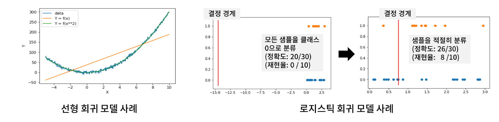
- Tip. 대다수의 머신러닝 모델은 선형식을 포함한다.
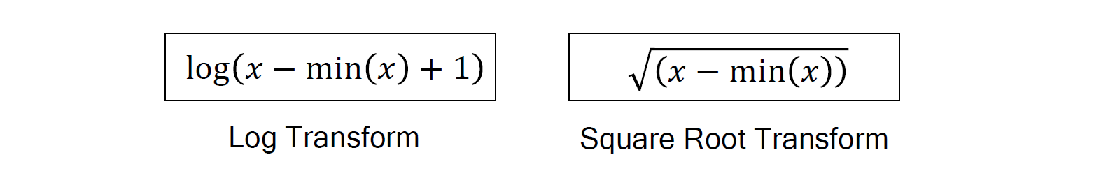
* 해결 방안
- 가장 이상적인 해결 방안은 각 특징에 대해, 특징과 라벨 간 관계를 나타내는 그래프를 통해 적절한 특징 변환을 수행해야 한다.
// 어떤 것이 좋을지 모르기 때문에 다 만들어서 확인을 해보는 것이다.
- 하지만 특징 개수가 많고, 다른 특징에 의한 영향도 존재하는 등 그래프를 통해 적절한 변환 방법을 선택하는 것은 쉽지 않아, 다양한 변환 방법을 사용하여 특징을 생성한 뒤 특징 선택을 수행해야 한다.
* 실습

// 5겹 교차 검증 기반의 평가를 수행한다.
// 로그와 제곱 관련 변수만 추가했을 뿐인데 성능이 좋아졌다.
// 특징을 선택을 할때 무조건 좋아 지는 것은 아니다.
[05. Part 5) Ch 19. 이상적인 분포를 만들순 없을까 변수 분포 문제 - 02. 이상치 제거 (1) IQR 규칙 활용]
* 문제 정의 및 해결 방안
- 변수 범위에서 많이 벗어난 아주 작은 값이나 아주 큰 값으로, 일반화된 모델을 생성하는데 악영향을 끼치는 값으로 이상치를 포함하는 레코드를 제거하는 방법으로 이상치를 제거한다. (절대 추정의 대상이 아님에 주의)

* 이상치 판단 방법 1. IQR 규칙 활용
- 변수별로 IQR 규칙을 만족하지 않는 샘플들을 판단하여 삭제 하는 방법

- 직관적이고 사용이 간편하다는 장점이 있지만, 단일 변수로 이상치를 판단하기 어려운 경우가 있다는 문제가 있다. (이전 페이지의 그림에서 표시된 이상치의 X 값은 이상치라고 보기 힘든 구간에 있었음에 주목한다.)
* numpy.quantile
- Array 의 q번째 quantile 을 구하는 함수
- 주요 입력
. a : input array (list, ndarray, array 등)
. q : quantile (0 과 1 사이)
* 실습

// 이상치가 있는 경우를 지워줘야 한다.
// 이상치의 비율이 30% 이상일 수는 없고, 1% 미만인것이 바람직하다.
// numpy.quantile Documentation
numpy.org/doc/stable/reference/generated/numpy.quantile.html
numpy.quantile(a, q, axis=None, out=None, overwrite_input=False, interpolation='linear', keepdims=False)
Compute the q-th quantile of the data along the specified axis.
New in version 1.15.0.
Parameters
aarray_like
Input array or object that can be converted to an array.
qarray_like of float
Quantile or sequence of quantiles to compute, which must be between 0 and 1 inclusive.
axis{int, tuple of int, None}, optional
Axis or axes along which the quantiles are computed. The default is to compute the quantile(s) along a flattened version of the array.
outndarray, optional
Alternative output array in which to place the result. It must have the same shape and buffer length as the expected output, but the type (of the output) will be cast if necessary.
overwrite_inputbool, optional
If True, then allow the input array a to be modified by intermediate calculations, to save memory. In this case, the contents of the input a after this function completes is undefined.
interpolation{‘linear’, ‘lower’, ‘higher’, ‘midpoint’, ‘nearest’}
This optional parameter specifies the interpolation method to use when the desired quantile lies between two data points i < j:
linear: i + (j - i) * fraction, where fraction is the fractional part of the index surrounded by i and j.
lower: i.
higher: j.
nearest: i or j, whichever is nearest.
midpoint: (i + j) / 2.
keepdimsbool, optional
If this is set to True, the axes which are reduced are left in the result as dimensions with size one. With this option, the result will broadcast correctly against the original array a.
Returns
quantilescalar or ndarray
If q is a single quantile and axis=None, then the result is a scalar. If multiple quantiles are given, first axis of the result corresponds to the quantiles. The other axes are the axes that remain after the reduction of a. If the input contains integers or floats smaller than float64, the output data-type is float64. Otherwise, the output data-type is the same as that of the input. If out is specified, that array is returned instead.
[05. Part 5) Ch 19. 이상적인 분포를 만들순 없을까 변수 분포 문제 - 03. 이상치 제거 (2) 밀도 기반 군집화 활용]
* 이상치 판단 방법 2. 밀도 기반 군집화 수행
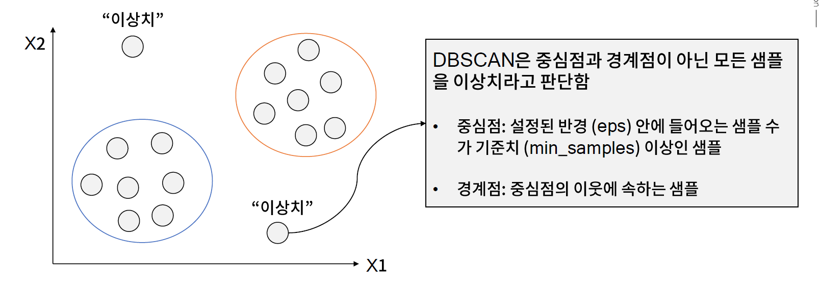
// 특정 반경내에서는 중심점.. 중심점에 안 들어오면 경계점 그 모두에 속하지 않는 것들이 이상치라고 부른다.
* sklearn.cluster.DBSCAN Documentation
scikit-learn.org/stable/modules/generated/sklearn.cluster.DBSCAN.html
class sklearn.cluster.DBSCAN(eps=0.5, *, min_samples=5, metric='euclidean', metric_params=None, algorithm='auto', leaf_size=30, p=None, n_jobs=None)Perform DBSCAN clustering from vector array or distance matrix.
DBSCAN - Density-Based Spatial Clustering of Applications with Noise. Finds core samples of high density and expands clusters from them. Good for data which contains clusters of similar density.
Read more in the User Guide.
Parameters
epsfloat, default=0.5
The maximum distance between two samples for one to be considered as in the neighborhood of the other. This is not a maximum bound on the distances of points within a cluster. This is the most important DBSCAN parameter to choose appropriately for your data set and distance function.
min_samplesint, default=5
The number of samples (or total weight) in a neighborhood for a point to be considered as a core point. This includes the point itself.
metricstring, or callable, default=’euclidean’
The metric to use when calculating distance between instances in a feature array. If metric is a string or callable, it must be one of the options allowed by sklearn.metrics.pairwise_distances for its metric parameter. If metric is “precomputed”, X is assumed to be a distance matrix and must be square. X may be a Glossary, in which case only “nonzero” elements may be considered neighbors for DBSCAN.
New in version 0.17: metric precomputed to accept precomputed sparse matrix.
metric_paramsdict, default=None
Additional keyword arguments for the metric function.
New in version 0.19.
algorithm{‘auto’, ‘ball_tree’, ‘kd_tree’, ‘brute’}, default=’auto’
The algorithm to be used by the NearestNeighbors module to compute pointwise distances and find nearest neighbors. See NearestNeighbors module documentation for details.
leaf_sizeint, default=30
Leaf size passed to BallTree or cKDTree. This can affect the speed of the construction and query, as well as the memory required to store the tree. The optimal value depends on the nature of the problem.
pfloat, default=None
The power of the Minkowski metric to be used to calculate distance between points.
n_jobsint, default=None
The number of parallel jobs to run. None means 1 unless in a joblib.parallel_backend context. -1 means using all processors. See Glossary for more details.
Attributes
core_sample_indices_ndarray of shape (n_core_samples,)
Indices of core samples.
components_ndarray of shape (n_core_samples, n_features)
Copy of each core sample found by training.
labels_ndarray of shape (n_samples)
Cluster labels for each point in the dataset given to fit(). Noisy samples are given the label -1.
* 실습

// cdist 은 DBSCAN 을 볼때 참고할 때를 위해서 가져온 library 이다.
// 파라미터를 조정하면서 값들을 확인한다.
[05. Part 5) Ch 19. 이상적인 분포를 만들순 없을까 변수 분포 문제 - 04. 특징 간 상관성 제거]

* 문제 정의
// 특징간 상관성이 높으면 강건한 파라미터 추정이 어렵다.

* 해결방법 (1) VIF 활용
// 다른 특징을 사용한 회귀 모델이 높은 R^2 을 보이는 경우

* 해결방법 (2) 주성분 분석
// 특징이 서로 직교

* sklearn.decomposition.PCA Documentation
scikit-learn.org/stable/modules/generated/sklearn.decomposition.PCA.html
class sklearn.decomposition.PCA(n_components=None, *, copy=True, whiten=False, svd_solver='auto', tol=0.0, iterated_power='auto', random_state=None)Principal component analysis (PCA).
Linear dimensionality reduction using Singular Value Decomposition of the data to project it to a lower dimensional space. The input data is centered but not scaled for each feature before applying the SVD.
It uses the LAPACK implementation of the full SVD or a randomized truncated SVD by the method of Halko et al. 2009, depending on the shape of the input data and the number of components to extract.
It can also use the scipy.sparse.linalg ARPACK implementation of the truncated SVD.
Notice that this class does not support sparse input. See TruncatedSVD for an alternative with sparse data.
Read more in the User Guide.
Parameters
n_componentsint, float, None or str
Number of components to keep. if n_components is not set all components are kept:
n_components == min(n_samples, n_features)
If n_components == 'mle' and svd_solver == 'full', Minka’s MLE is used to guess the dimension. Use of n_components == 'mle' will interpret svd_solver == 'auto' as svd_solver == 'full'.
If 0 < n_components < 1 and svd_solver == 'full', select the number of components such that the amount of variance that needs to be explained is greater than the percentage specified by n_components.
If svd_solver == 'arpack', the number of components must be strictly less than the minimum of n_features and n_samples.
Hence, the None case results in:
n_components == min(n_samples, n_features) - 1
copybool, default=True
If False, data passed to fit are overwritten and running fit(X).transform(X) will not yield the expected results, use fit_transform(X) instead.
whitenbool, optional (default False)
When True (False by default) the components_ vectors are multiplied by the square root of n_samples and then divided by the singular values to ensure uncorrelated outputs with unit component-wise variances.
Whitening will remove some information from the transformed signal (the relative variance scales of the components) but can sometime improve the predictive accuracy of the downstream estimators by making their data respect some hard-wired assumptions.
svd_solverstr {‘auto’, ‘full’, ‘arpack’, ‘randomized’}If auto :
The solver is selected by a default policy based on X.shape and n_components: if the input data is larger than 500x500 and the number of components to extract is lower than 80% of the smallest dimension of the data, then the more efficient ‘randomized’ method is enabled. Otherwise the exact full SVD is computed and optionally truncated afterwards.
If full :
run exact full SVD calling the standard LAPACK solver via scipy.linalg.svd and select the components by postprocessing
If arpack :
run SVD truncated to n_components calling ARPACK solver via scipy.sparse.linalg.svds. It requires strictly 0 < n_components < min(X.shape)
If randomized :
run randomized SVD by the method of Halko et al.
New in version 0.18.0.
tolfloat >= 0, optional (default .0)
Tolerance for singular values computed by svd_solver == ‘arpack’.
New in version 0.18.0.
iterated_powerint >= 0, or ‘auto’, (default ‘auto’)
Number of iterations for the power method computed by svd_solver == ‘randomized’.
New in version 0.18.0.
random_stateint, RandomState instance, default=None
Used when svd_solver == ‘arpack’ or ‘randomized’. Pass an int for reproducible results across multiple function calls. See Glossary.
New in version 0.18.0.
Attributes
components_array, shape (n_components, n_features)
Principal axes in feature space, representing the directions of maximum variance in the data. The components are sorted by explained_variance_.
explained_variance_array, shape (n_components,)
The amount of variance explained by each of the selected components.
Equal to n_components largest eigenvalues of the covariance matrix of X.
New in version 0.18.
explained_variance_ratio_array, shape (n_components,)
Percentage of variance explained by each of the selected components.
If n_components is not set then all components are stored and the sum of the ratios is equal to 1.0.
singular_values_array, shape (n_components,)
The singular values corresponding to each of the selected components. The singular values are equal to the 2-norms of the n_components variables in the lower-dimensional space.
New in version 0.19.
mean_array, shape (n_features,)
Per-feature empirical mean, estimated from the training set.
Equal to X.mean(axis=0).
n_components_int
The estimated number of components. When n_components is set to ‘mle’ or a number between 0 and 1 (with svd_solver == ‘full’) this number is estimated from input data. Otherwise it equals the parameter n_components, or the lesser value of n_features and n_samples if n_components is None.
n_features_int
Number of features in the training data.
n_samples_int
Number of samples in the training data.
noise_variance_float
The estimated noise covariance following the Probabilistic PCA model from Tipping and Bishop 1999. See “Pattern Recognition and Machine Learning” by C. Bishop, 12.2.1 p. 574 or http://www.miketipping.com/papers/met-mppca.pdf. It is required to compute the estimated data covariance and score samples.
Equal to the average of (min(n_features, n_samples) - n_components) smallest eigenvalues of the covariance matrix of X.
* 실습

// 특징간 상관 관계가 너무 크다.
// VIF 계산. LinearRegression 으로 작업한 후 R sqaure

// PCA 를 활용
[05. Part 5) Ch 19. 이상적인 분포를 만들순 없을까 변수 분포 문제 - 05. 변수 치우침 제거]
* 문제 정의
// 치우친 반대 방향의 값(꼬리 부분) 들이 이상치 처럼 작용할 가능성이 크다.

* 탐색 방법 : 왜도(skewness)
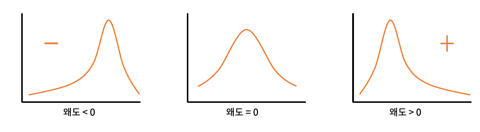
// 왜도의 절대값이 1.5이상 이면 치우쳤다고 판단할 수 있다.
* scipy.stats
- scipy.stats.mode
- scipy.stats.skew
- scipy.stats.kurtosis
* 해결방안
* 실습
// scipy.stats.mode Documentation
docs.scipy.org/doc/scipy/reference/generated/scipy.stats.mode.html
scipy.stats.mode(a, axis=0, nan_policy='propagate')[source]Return an array of the modal (most common) value in the passed array.
If there is more than one such value, only the smallest is returned. The bin-count for the modal bins is also returned.
Parameters
aarray_like
n-dimensional array of which to find mode(s).
axisint or None, optional
Axis along which to operate. Default is 0. If None, compute over the whole array a.
nan_policy{‘propagate’, ‘raise’, ‘omit’}, optional
Defines how to handle when input contains nan. The following options are available (default is ‘propagate’):
‘propagate’: returns nan
‘raise’: throws an error
‘omit’: performs the calculations ignoring nan values
Returns
modendarray
Array of modal values.
countndarray
Array of counts for each mode.
//scipy.stats.skew Documentation
docs.scipy.org/doc/scipy/reference/generated/scipy.stats.skew.html
scipy.stats.skew(a, axis=0, bias=True, nan_policy='propagate')[source]Compute the sample skewness of a data set.
For normally distributed data, the skewness should be about zero. For unimodal continuous distributions, a skewness value greater than zero means that there is more weight in the right tail of the distribution. The function skewtest can be used to determine if the skewness value is close enough to zero, statistically speaking.
Parameters
andarray
Input array.
axisint or None, optional
Axis along which skewness is calculated. Default is 0. If None, compute over the whole array a.
biasbool, optional
If False, then the calculations are corrected for statistical bias.
nan_policy{‘propagate’, ‘raise’, ‘omit’}, optional
Defines how to handle when input contains nan. The following options are available (default is ‘propagate’):
‘propagate’: returns nan
‘raise’: throws an error
‘omit’: performs the calculations ignoring nan values
Returns
skewnessndarray
The skewness of values along an axis, returning 0 where all values are equal.
// scipy.stats.kurtosis Documentation
docs.scipy.org/doc/scipy/reference/generated/scipy.stats.kurtosis.html
scipy.stats.kurtosis(a, axis=0, fisher=True, bias=True, nan_policy='propagate')[source]Compute the kurtosis (Fisher or Pearson) of a dataset.
Kurtosis is the fourth central moment divided by the square of the variance. If Fisher’s definition is used, then 3.0 is subtracted from the result to give 0.0 for a normal distribution.
If bias is False then the kurtosis is calculated using k statistics to eliminate bias coming from biased moment estimators
Use kurtosistest to see if result is close enough to normal.
Parameters
aarray
Data for which the kurtosis is calculated.
axisint or None, optional
Axis along which the kurtosis is calculated. Default is 0. If None, compute over the whole array a.
fisherbool, optional
If True, Fisher’s definition is used (normal ==> 0.0). If False, Pearson’s definition is used (normal ==> 3.0).
biasbool, optional
If False, then the calculations are corrected for statistical bias.
nan_policy{‘propagate’, ‘raise’, ‘omit’}, optional
Defines how to handle when input contains nan. ‘propagate’ returns nan, ‘raise’ throws an error, ‘omit’ performs the calculations ignoring nan values. Default is ‘propagate’.
Returns
kurtosisarray
The kurtosis of values along an axis. If all values are equal, return -3 for Fisher’s definition and 0 for Pearson’s definition.
[05. Part 5) Ch 19. 이상적인 분포를 만들순 없을까 변수 분포 문제 - 06. 스케일링]

* 문제 정의
// 특징간 스케일이 달라서 발생하는 문제이다.
// 거리 기반 모델 -> 스케일이 큰 변수에 영향을 받는 모델
// 작은것 -> 회귀모델, 서포트 벡터 머신, 신경망
// 영향이 없는 것 -> 나이브베이즈 의사결정나무
* 해결방법
// 스케일을 줄이는 것!

// standard Scaling 보다는 Min_max 스케일링이 좀 더 맞다고 본다.
* sklearn.preprocessing.MinMaxScaler & StandardScaler Documentation
- sklearn.preprocessing.MinMaxScaler
scikit-learn.org/stable/modules/generated/sklearn.preprocessing.MinMaxScaler.html
class sklearn.preprocessing.MinMaxScaler(feature_range=(0, 1), *, copy=True)Transform features by scaling each feature to a given range.
This estimator scales and translates each feature individually such that it is in the given range on the training set, e.g. between zero and one.
The transformation is given by:
X_std = (X - X.min(axis=0)) / (X.max(axis=0) - X.min(axis=0)) X_scaled = X_std * (max - min) + min
where min, max = feature_range.
This transformation is often used as an alternative to zero mean, unit variance scaling.
Read more in the User Guide.
Parameters
feature_rangetuple (min, max), default=(0, 1)
Desired range of transformed data.
copybool, default=True
Set to False to perform inplace row normalization and avoid a copy (if the input is already a numpy array).
Attributes
min_ndarray of shape (n_features,)
Per feature adjustment for minimum. Equivalent to min - X.min(axis=0) * self.scale_
scale_ndarray of shape (n_features,)
Per feature relative scaling of the data. Equivalent to (max - min) / (X.max(axis=0) - X.min(axis=0))
New in version 0.17: scale_ attribute.
data_min_ndarray of shape (n_features,)
Per feature minimum seen in the data
New in version 0.17: data_min_
data_max_ndarray of shape (n_features,)
Per feature maximum seen in the data
New in version 0.17: data_max_
data_range_ndarray of shape (n_features,)
Per feature range (data_max_ - data_min_) seen in the data
New in version 0.17: data_range_
n_samples_seen_int
The number of samples processed by the estimator. It will be reset on new calls to fit, but increments across partial_fit calls.
- sklearn.preprocessing.MinMaxScaler
scikit-learn.org/stable/modules/generated/sklearn.preprocessing.StandardScaler.html
class sklearn.preprocessing.StandardScaler(*, copy=True, with_mean=True, with_std=True)Standardize features by removing the mean and scaling to unit variance
The standard score of a sample x is calculated as:
z = (x - u) / s
where u is the mean of the training samples or zero if with_mean=False, and s is the standard deviation of the training samples or one if with_std=False.
Centering and scaling happen independently on each feature by computing the relevant statistics on the samples in the training set. Mean and standard deviation are then stored to be used on later data using transform.
Standardization of a dataset is a common requirement for many machine learning estimators: they might behave badly if the individual features do not more or less look like standard normally distributed data (e.g. Gaussian with 0 mean and unit variance).
For instance many elements used in the objective function of a learning algorithm (such as the RBF kernel of Support Vector Machines or the L1 and L2 regularizers of linear models) assume that all features are centered around 0 and have variance in the same order. If a feature has a variance that is orders of magnitude larger that others, it might dominate the objective function and make the estimator unable to learn from other features correctly as expected.
This scaler can also be applied to sparse CSR or CSC matrices by passing with_mean=False to avoid breaking the sparsity structure of the data.
Read more in the User Guide.
Parameters
copyboolean, optional, default True
If False, try to avoid a copy and do inplace scaling instead. This is not guaranteed to always work inplace; e.g. if the data is not a NumPy array or scipy.sparse CSR matrix, a copy may still be returned.
with_meanboolean, True by default
If True, center the data before scaling. This does not work (and will raise an exception) when attempted on sparse matrices, because centering them entails building a dense matrix which in common use cases is likely to be too large to fit in memory.
with_stdboolean, True by default
If True, scale the data to unit variance (or equivalently, unit standard deviation).
Attributes
scale_ndarray or None, shape (n_features,)
Per feature relative scaling of the data. This is calculated using np.sqrt(var_). Equal to None when with_std=False.
New in version 0.17: scale_
mean_ndarray or None, shape (n_features,)
The mean value for each feature in the training set. Equal to None when with_mean=False.
var_ndarray or None, shape (n_features,)
The variance for each feature in the training set. Used to compute scale_. Equal to None when with_std=False.
n_samples_seen_int or array, shape (n_features,)
The number of samples processed by the estimator for each feature. If there are not missing samples, the n_samples_seen will be an integer, otherwise it will be an array. Will be reset on new calls to fit, but increments across partial_fit calls.
[파이썬을 활용한 데이터 전처리 Level UP-Comment]
- 범주형 변수 문자에 대한 처리 방법
- 이상적인 분포형에 대한 내용... 특히 스케일링. 이건 잘해야지~
파이썬을 활용한 데이터 전처리 Level UP 올인원 패키지 Online. | 패스트캠퍼스
데이터 분석에 필요한 기초 전처리부터, 데이터의 품질 및 머신러닝 성능 향상을 위한 고급 스킬까지 완전 정복하는 데이터 전처리 트레이닝 온라인 강의입니다.
www.fastcampus.co.kr
'Programming > Python' 카테고리의 다른 글
| 패스트캠퍼스 파이썬을 활용한 데이터 전처리 Level UP 챌린지 참여 후기 (0) | 2020.12.08 |
|---|---|
| [패스트캠퍼스 수강 후기] 데이터전처리 100% 환급 챌린지 28회차 미션 (0) | 2020.11.29 |
| [패스트캠퍼스 수강 후기] 데이터전처리 100% 환급 챌린지 26회차 미션 (0) | 2020.11.27 |
| [패스트캠퍼스 수강 후기] 데이터전처리 100% 환급 챌린지 25회차 미션 (0) | 2020.11.26 |
| [패스트캠퍼스 수강 후기] 데이터전처리 100% 환급 챌린지 24회차 미션 (0) | 2020.11.25 |